Glacier flowlines
Centerlines
Computing the centerlines is the first task to run after the definition of the local map and topography.
Our algorithm is an implementation of the procedure described by Kienholz et al., (2014). Appart from some minor changes (mostly the choice of certain parameters), we stayed close to the original algorithm.
The basic idea is to find the terminus of the glacier (its lowest point) and a series of flowline “heads” (local elevation maxima). The centerlines are then computed with a least cost routing algorithm minimizing both (i) the total elevation gain and (ii) the distance from the glacier outline:
In [1]: graphics.plot_centerlines(gdir)

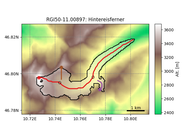
The glacier has a major centerline (the longest one), and tributary branches (in this case: two).
At this stage, the centerlines are still not fully suitable for modelling. Therefore, a rather simple procedure converts them to “flowlines”, which now have a regular coordinate spacing (which they will keep for the rest of the workflow). The tail of the tributaries are cut according to a distance threshold rule:
In [2]: graphics.plot_centerlines(gdir, use_flowlines=True)
Downstream lines
For the glacier to be able to grow we need to determine the flowlines downstream of the current glacier geometry:
In [3]: graphics.plot_centerlines(gdir, use_flowlines=True, add_downstream=True)

The downsteam lines area also computed using a routing algorithm minimizing the distance between the glacier terminus and the border of the map as well as the total elevation gain, therefore following the valley floor.
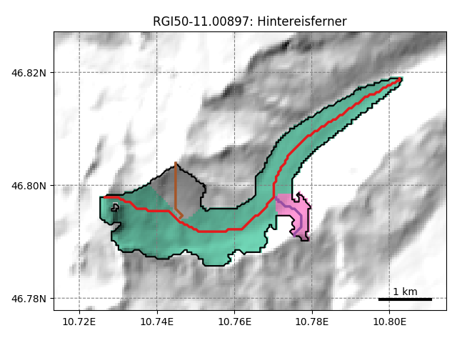
Catchment areas
Each flowline has its own “catchment area”. These areas are computed using similar flow routing methods as the one used for determining the flowlines. Their purpose is to attribute each glacier pixel to the right tributory in order to compute mass gain and loss for each tributary. This will also influence the later computation of the glacier widths).
In [4]: tasks.catchment_area(gdir)

In [5]: graphics.plot_catchment_areas(gdir)
Flowline widths
Finally, the flowline widths are computed in two steps.
First, we compute the geometrical width at each grid point. The width is drawn from the intersection of a line perpendicular to the flowline and either (i) the glacier outlines or (ii) the catchment boundaries:
In [6]: tasks.catchment_width_geom(gdir)

In [7]: graphics.plot_catchment_width(gdir)
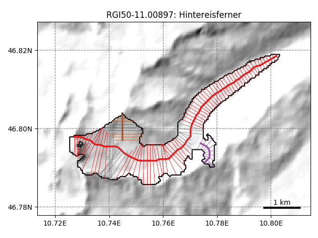
Then, these geometrical widths are corrected so that the altitude-area distribution of the “flowline-glacier” is as close as possible as the actual distribution of the glacier using its full 2D geometry:
In [8]: tasks.catchment_width_correction(gdir)

In [9]: graphics.plot_catchment_width(gdir, corrected=True)

Note that a perfect match is not possible since the sample size is not the same between the “1.5D” and the 2D representation of the glacier.
Implementation details
Shared setup for these examples:
import geopandas as gpd
import oggm
from oggm import cfg, tasks
from oggm.utils import get_demo_file, gettempdir

cfg.initialize()
cfg.set_intersects_db(get_demo_file('rgi_intersect_oetztal.shp'))
cfg.PATHS['dem_file'] = get_demo_file('hef_srtm.tif')

base_dir = gettempdir('Flowlines_Docs')
cfg.PATHS['working_dir'] = base_dir
entity = gpd.read_file(get_demo_file('HEF_MajDivide.shp')).iloc[0]
gdir = oggm.GlacierDirectory(entity, base_dir=base_dir, reset=True)

tasks.define_glacier_region(gdir, entity=entity)
tasks.glacier_masks(gdir)
tasks.compute_centerlines(gdir)
tasks.initialize_flowlines(gdir)
tasks.compute_downstream_line(gdir)