1. Set-up a default run for a list of glaciers

This example shows how to run the OGGM model for a list of selected glaciers (here, four). For this example we download the list of glaciers from Fabien’s dropbox, but you can use any list of glaciers for this. See the prepare_glacier_list.ipynb notebook in the oggm/docs/notebooks directory for an example on how to prepare such a file.

Note that the default in OGGM is to use a previously calibrated list of \(t^*\) for the run, which means that we don’t have to calibrate the mass balance model ourselves (thankfully, otherwise you would have to add all the calibration glaciers to your list too).

Note that to be exact, this procedure can only be applied if the model parameters don’t change between the calibration and the run. After testing, it appears that changing the ‘border’ parameter won’t affect the results much (as expected), so it’s ok to change this parameter. Some other parameters (e.g. topo smoothing, dx, precip factor, alternative climate data…) will probably need a re-calibration (see the OGGM calibration recipe for this).

Script

# Python imports
from os import path
import shutil
import zipfile
import oggm

# Module logger
import logging
log = logging.getLogger(__name__)

# Libs
import salem

# Locals
import oggm.cfg as cfg
from oggm import tasks, utils, workflow
from oggm.workflow import execute_entity_task

# For timing the run
import time
start = time.time()

# Initialize OGGM and set up the default run parameters
cfg.initialize()

# Local working directory (where OGGM will write its output)
WORKING_DIR = path.join(path.expanduser('~'), 'tmp', 'OGGM_precalibrated_run')
utils.mkdir(WORKING_DIR, reset=True)
cfg.PATHS['working_dir'] = WORKING_DIR

# Use multiprocessing?
cfg.PARAMS['use_multiprocessing'] = True

# Here we override some of the default parameters
# How many grid points around the glacier?
# Make it large if you expect your glaciers to grow large
cfg.PARAMS['border'] = 100

# Set to True for operational runs
cfg.PARAMS['continue_on_error'] = False

# We use intersects
# (this is slow, it could be replaced with a subset of the global file)
rgi_dir = utils.get_rgi_intersects_dir(version='5')
cfg.set_intersects_db(path.join(rgi_dir, '00_rgi50_AllRegs',
                                'intersects_rgi50_AllRegs.shp'))

# Pre-download other files which will be needed later
utils.get_cru_cl_file()
utils.get_cru_file(var='tmp')
utils.get_cru_file(var='pre')

# Download the RGI file for the run
# We us a set of four glaciers here but this could be an entire RGI region,
# or any glacier list you'd like to model
dl = 'https://www.dropbox.com/s/6cwi7b4q4zqgh4a/RGI_example_glaciers.zip?dl=1'
with zipfile.ZipFile(utils.file_downloader(dl)) as zf:
    zf.extractall(WORKING_DIR)
rgidf = salem.read_shapefile(path.join(WORKING_DIR, 'RGI_example_glaciers',
                                       'RGI_example_glaciers.shp'))

# Sort for more efficient parallel computing
rgidf = rgidf.sort_values('Area', ascending=False)

log.info('Starting OGGM run')
log.info('Number of glaciers: {}'.format(len(rgidf)))

# Go - initialize working directories
gdirs = workflow.init_glacier_regions(rgidf)

# Preprocessing tasks
task_list = [
    tasks.glacier_masks,
    tasks.compute_centerlines,
    tasks.initialize_flowlines,
    tasks.compute_downstream_line,
    tasks.compute_downstream_bedshape,
    tasks.catchment_area,
    tasks.catchment_intersections,
    tasks.catchment_width_geom,
    tasks.catchment_width_correction,
]
for task in task_list:
    execute_entity_task(task, gdirs)

# Climate tasks -- only data IO and tstar interpolation!
execute_entity_task(tasks.process_cru_data, gdirs)
tasks.distribute_t_stars(gdirs)
execute_entity_task(tasks.apparent_mb, gdirs)

# Inversion tasks
execute_entity_task(tasks.prepare_for_inversion, gdirs)
# We use the default parameters for this run
execute_entity_task(tasks.volume_inversion, gdirs, glen_a=cfg.A, fs=0)
execute_entity_task(tasks.filter_inversion_output, gdirs)

# Final preparation for the run
execute_entity_task(tasks.init_present_time_glacier, gdirs)

# Random climate representative for the tstar climate, without bias
# In an ideal world this would imply that the glaciers remain stable,
# but it doesn't have to be so
execute_entity_task(tasks.random_glacier_evolution, gdirs,
                    nyears=200, bias=0, seed=1,
                    filesuffix='_tstar')

# Compile output
log.info('Compiling output')
utils.glacier_characteristics(gdirs)
utils.compile_run_output(gdirs, filesuffix='_tstar')

# Log
m, s = divmod(time.time() - start, 60)
h, m = divmod(m, 60)
log.info('OGGM is done! Time needed: %d:%02d:%02d' % (h, m, s))

If everything went well, you should see an output similar to:

2017-10-21 00:07:17: oggm.cfg: Parameter file: /home/mowglie/Documents/git/oggm-fork/oggm/params.cfg
2017-10-21 00:07:27: __main__: Starting OGGM run
2017-10-21 00:07:27: __main__: Number of glaciers: 4
2017-10-21 00:07:27: oggm.workflow: Multiprocessing: using all available processors (N=4)
2017-10-21 00:07:27: oggm.core.gis: (RGI50-01.10299) define_glacier_region
2017-10-21 00:07:27: oggm.core.gis: (RGI50-18.02342) define_glacier_region
(...)
2017-10-21 00:09:30: oggm.core.flowline: (RGI50-01.10299) default time stepping was successful!
2017-10-21 00:09:39: oggm.core.flowline: (RGI50-18.02342) default time stepping was successful!
2017-10-21 00:09:39: __main__: Compiling output
2017-10-21 00:09:39: __main__: OGGM is done! Time needed: 0:02:22

Note

During the random_glacier_evolution task some numerical warnings might occur. These are expected to happen and are caught by the solver, which then tries a more conservative time stepping scheme.

Note

The random_glacier_evolution task can be replaced by any climate scenario built by the user. For this you’ll have to develop your own task, which will be the topic of another example script.

Starting from a preprocessed state

Now that we’ve gone through all the preprocessing steps once and that their output is stored on disk, it isn’t necessary to re-run everything to make a new experiment. The code can be simplified to:

# Python imports
from os import path
import oggm

# Module logger
import logging
log = logging.getLogger(__name__)

# Libs
import salem

# Locals
import oggm.cfg as cfg
from oggm import tasks, utils, workflow
from oggm.workflow import execute_entity_task

# For timing the run
import time
start = time.time()

# Initialize OGGM and set up the run parameters
cfg.initialize()

# Local working directory (where OGGM will write its output)
WORKING_DIR = path.join(path.expanduser('~'), 'tmp', 'OGGM_precalibrated_run')
cfg.PATHS['working_dir'] = WORKING_DIR

# Use multiprocessing?
cfg.PARAMS['use_multiprocessing'] = True

# Read RGI
rgidf = salem.read_shapefile(path.join(WORKING_DIR, 'RGI_example_glaciers',
                                       'RGI_example_glaciers.shp'))
# Sort for more efficient parallel computing
rgidf = rgidf.sort_values('Area', ascending=False)

log.info('Starting OGGM run')
log.info('Number of glaciers: {}'.format(len(rgidf)))

# Initialize from existing directories
gdirs = workflow.init_glacier_regions(rgidf)

# We can step directly to a new experiment!
# Random climate representative for the recent climate (1985-2015)
# This is a kinf of "commitment" run
execute_entity_task(tasks.random_glacier_evolution, gdirs,
                    nyears=200, y0=2000, seed=1,
                    filesuffix='_commitment')

# Compile output
log.info('Compiling output')
utils.compile_run_output(gdirs, filesuffix='_commitment')

# Log
m, s = divmod(time.time() - start, 60)
h, m = divmod(m, 60)
log.info('OGGM is done! Time needed: %d:%02d:%02d' % (h, m, s))

Note

Note the use of the filesuffix keyword argument. This allows to store the output of different runs in different files, useful for later analyses.

Some analyses

The output directory contains the compiled output files from the run. The glacier_characteristics.csv file contains various information about each glacier obation after the preprocessing, either from the RGI directly (location, name, glacier type…) or from the model itself (hypsometry, inversion model output…).

Here is an example of how to read the file:

from os import path
import pandas as pd
WORKING_DIR = path.join(path.expanduser('~'), 'tmp', 'OGGM_precalibrated_run')
df = pd.read_csv(path.join(WORKING_DIR, 'glacier_characteristics.csv'))
print(df)

Output (reduced for clarity):

rgi_id	name	cenlon	cenlat	rgi_area_km2	terminus_type	dem_max_elev	dem_min_elev	n_centerlines	longuest_centerline_km	inv_thickness_m	vas_thickness_m
RGI50-18.02342	Tasman Glacier	170.238	-43.5653	95.216	Land-terminating	3662	715	7	27.2195	186.38	187.713
RGI50-01.10299	Coxe Glacier	-148.037	61.144	19.282	Marine-terminating	1840	6	8	11.6243	137.153	103.136
RGI50-11.00897	Hintereisferner	10.7584	46.8003	8.036	Land-terminating	3684	2447	3	8.99975	107.642	74.2795
RGI50-08.02637	Storglaciaeren	18.5604	67.9042	3.163	Land-terminating	1909	1176	2	3.54495	63.2469	52.362

The run outpout is stored in netCDF files, and it can therefore be read with any tool able to read those (Matlab, R, …).

I myself am familiar with python, and I use the xarray package to read the data:

import xarray as xr
import matplotlib.pyplot as plt
from os import path

WORKING_DIR = path.join(path.expanduser('~'), 'tmp', 'OGGM_precalibrated_run')
ds1 = xr.open_dataset(path.join(WORKING_DIR, 'run_output_tstar.nc'))
ds2 = xr.open_dataset(path.join(WORKING_DIR, 'run_output_commitment.nc'))

v1_km3 = ds1.volume * 1e-9
v2_km3 = ds2.volume * 1e-9
l1_km = ds1.length * 1e-3
l2_km = ds2.length * 1e-3

f, axs = plt.subplots(2, 4, figsize=(12, 4), sharex=True)

for i in range(4):
    ax = axs[0, i]
    v1_km3.isel(rgi_id=i).plot(ax=ax, label='t*')
    v2_km3.isel(rgi_id=i).plot(ax=ax, label='Commitment')
    if i == 0:
        ax.set_ylabel('Volume [km3]')
        ax.legend(loc='best')
    else:
        ax.set_ylabel('')
    ax.set_xlabel('')

    ax = axs[1, i]

    # Length can need a bit of postprocessing because of some cold years
    # Where seasonal snow is thought to be a glacier...
    for l in [l1_km, l2_km]:
        roll_yrs = 5
        sel = l.isel(rgi_id=i).to_series()
        # Take the minimum out of 5 years
        sel = sel.rolling(roll_yrs).min()
        sel.iloc[0:roll_yrs] = sel.iloc[roll_yrs]
        sel.plot(ax=ax)
    if i == 0:
        ax.set_ylabel('Length [m]')
    else:
        ax.set_ylabel('')
    ax.set_xlabel('Years')
    ax.set_title('')

plt.tight_layout()
plt.show()

This code snippet should produce the following plot:

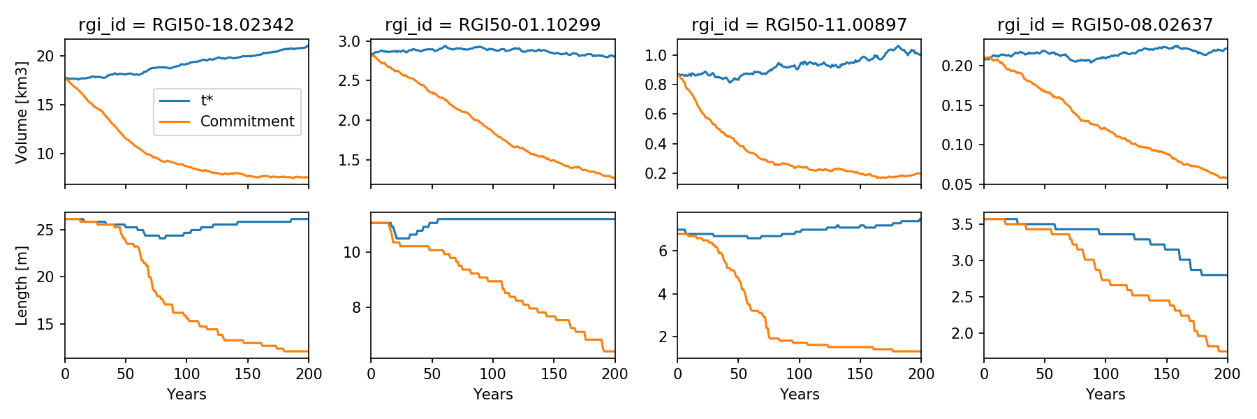
Warning

In the script above we have to “smooth” our length data for nicer plots. This is necessary because of annual snow cover: indeed, OGGM cannot differentiate between snow and ice. At the end of a cold mass-balance year, it can happen that some snow remains at the tongue and below: for the model, this looks like a longer glacier… (this cover is very thin, so that it doesn’t influence the volume much).

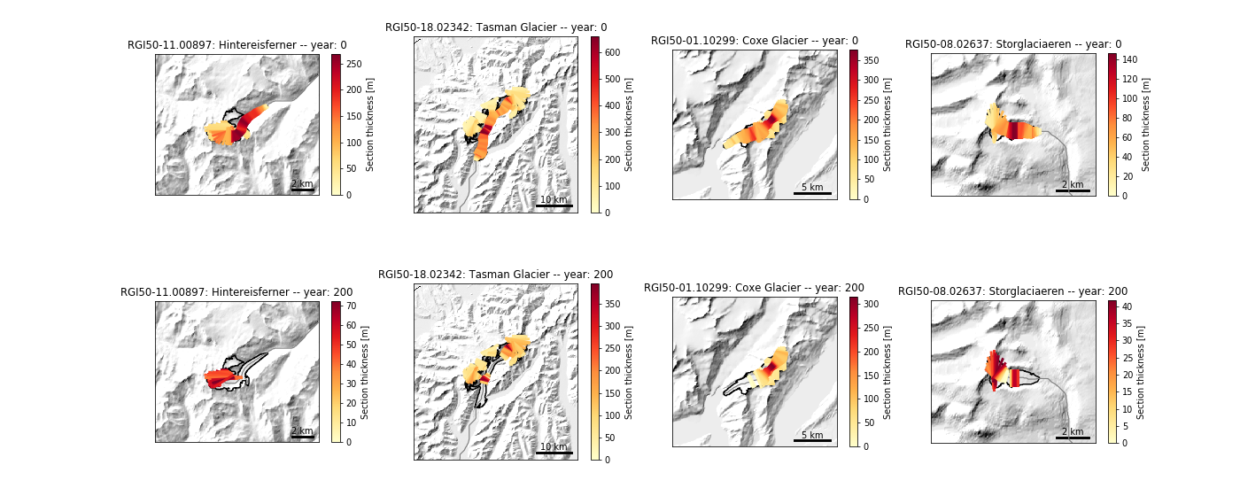
More analyses

Here is a more complex example to demonstrate how to plot the glacier geometries after the run:

# Python imports
import logging
from os import path

# External modules
import matplotlib.pyplot as plt

# Locals
import oggm.cfg as cfg
from oggm import workflow, graphics
from oggm.core import flowline

# Module logger
log = logging.getLogger(__name__)

# Initialize OGGM
cfg.initialize()

# Local working directory (where OGGM will write its output)
WORKING_DIR = path.join(path.expanduser('~'), 'tmp', 'OGGM_precalibrated_run')
cfg.PATHS['working_dir'] = WORKING_DIR

# Initialize from existing directories
# (note that we don't need the RGI file: this is going to be slow sometimes
# but it works)
gdirs = workflow.init_glacier_regions()

# Plot: we will show the state of all four glaciers at the beginning and at
# the end of the commitment simulation
f, axs = plt.subplots(2, 4, figsize=(20, 8))

for i in range(4):
    ax = axs[0, i]
    gdir = gdirs[i]
    # Use the model ouptut file to simulate the glacier evolution
    model = flowline.FileModel(gdir.get_filepath('model_run',
                                                 filesuffix='_commitment'))
    graphics.plot_modeloutput_map(gdirs[i], model=model, ax=ax,
                                  lonlat_contours_kwargs={'interval': 0})
    ax = axs[1, i]
    model.run_until(200)
    graphics.plot_modeloutput_map(gdirs[i], model=model, ax=ax,
                                  lonlat_contours_kwargs={'interval': 0})

plt.subplots_adjust(wspace=0.4, hspace=0.08, top=0.98, bottom=0.02)
plt.show()

Which should produce the following plot: