Bed inversion
To compute the initial ice thickness \(h_0\), OGGM follows a methodology largely inspired from [Farinotti_etal_2009], but fully automatised and relying on different methods for the mass-balance and the calibration.
Basics
The principle is simple. Let’s assume for now that we know the flux of ice \(q\) flowing through a section of our glacier. The flowline physics and geometrical assumptions can be used to solve for the ice thickness \(h\):
With \(n=3\) and \(S = h w\) (in the case of a rectangular section) or \(S = 2 / 3 h w\) (parabolic section), the equation reduces to solving a polynomial of degree 5 with one unique solution in \(\mathbb{R}_+\). If we neglect sliding (the default in OGGM and in [Farinotti_etal_2009]), the solution is even simpler.
Ice flux
If we consider a point on the flowline and the catchment area \(\Omega\) upstream of this point we have:
with \(\dot{m}\) the mass balance, and \(\widetilde{m} = \dot{m} - \rho \partial h / \partial t\) the “apparent mass-balance” after [Farinotti_etal_2009]. If the glacier is in steady state, the apparent mass-balance is equivalent to the the actual (and observable) mass-balance. Unfortunately, \(\partial h / \partial t\) is not known and there is no easy way to compute it. In order to continue, we have to make the assumption that our geometry is in equilibrium.
This however has a very useful consequence: indeed, for the calibration of our Mass-balance model it is required to find a date \(t^*\) at which the glacier would be in equilibrium with its average climate while conserving its modern geometry. Thus, we have \(\widetilde{m} = \dot{m}_{t^*}\), where \(\dot{m}_{t^*}\) is the 31-yr average mass-balance centered at \(t^*\) (which is known since the mass-balance model calibration).
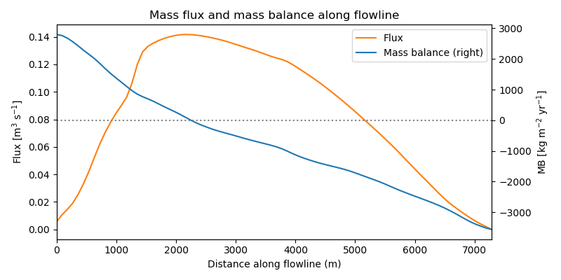
The plot below shows the mass flux along the major flowline of Hintereisferner glacier. By construction, the flux is maximal at the equilibrium line and zero at the glacier tongue.
In [1]: example_plot_massflux()
Calibration
A number of climate and glacier related parameters are fixed prior to the inversion, leaving only one free parameter for the calibration of the bed inversion procedure: the inversion factor \(f_{inv}\). It is defined such as:
With \(A_0\) the standard creep parameter (2.4e-24). Currently, \(f_{inv}\) is calibrated to minimize the volume RMSD of all glaciers with a volume estimation in the GlaThiDa database. It is therefore neither glacier nor temperature dependent and does not account for uncertainties in GlaThiDa’s glacier-wide thickness estimations, two approximations which should be better handled in the future.
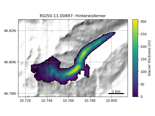
Distributed ice thickness
To obtain a 2D map of the glacier bed, the flowline thicknesses need to be interpolated to the glacier mask. The current implementation of this step in OGGM is currently very simple, but provides nice looking maps:
In [2]: tasks.catchment_area(gdir)

In [3]: graphics.plot_distributed_thickness(gdir)
References
| [Cuffey_Paterson_2010] | Cuffey, K., and W. S. B. Paterson (2010). The Physics of Glaciers, Butterworth‐Heinemann, Oxford, U.K. |
| [Farinotti_etal_2009] | (1, 2, 3) Farinotti, D., Huss, M., Bauder, A., Funk, M., & Truffer, M. (2009). A method to estimate the ice volume and ice-thickness distribution of alpine glaciers. Journal of Glaciology, 55 (191), 422–430. |
| [Golledge_Levy_2011] | Golledge, N. R., and Levy, R. H. (2011). Geometry and dynamics of an East Antarctic Ice Sheet outlet glacier, under past and present climates. Journal of Geophysical Research: Earth Surface, 116(3), 1–13. |
| [Jarosch_etal_2013] | Jarosch, a. H., Schoof, C. G., & Anslow, F. S. (2013). Restoring mass conservation to shallow ice flow models over complex terrain. Cryosphere, 7(1), 229–240. http://doi.org/10.5194/tc-7-229-2013 |
| [Oerlemans_1997] | Oerlemans, J. (1997). A flowline model for Nigardsbreen, Norway: projection of future glacier length based on dynamic calibration with the historic record. Journal of Glaciology, 24, 382–389. |