Input data
OGGM needs various data files to run. Currently, we rely exclusively on open-access data that are all downloaded automatically for the user. This page explains the various ways OGGM uses to get to the data it needs.
First, you will have to set-up your System settings (you’ll need to do this only once per computer). Then, we recommend to start your runs from Pre-processed directories: these are ready-to-run Glacier directories at various levels of pre-processing state, thus reducing the amount of pre-processing you’ll have to do yourself. It is also possible to do a full run “from scratch”, in which case OGGM will download the Raw data sources for you as well.
System settings
OGGM implements a bunch of tools to make access to the input data as painless as possible for you, including the automated download of all the required files. This requires you to tell OGGM where to store these data.
Calibration data and testing: the ~/.oggm directory
At the first import, OGGM will create a cached .oggm directory in your
$HOME folder. This directory contains all data obtained from the
oggm sample data repository. It contains several files needed only for
testing, but also some important files needed for calibration and validation.
For example:
- The CRU baseline climatology (CL v2.0, obtained from crudata.uea.ac.uk/ and prepared for OGGM),
- The reference mass-balance data from WGMS with links to the respective RGI polygons,
- The reference ice thickness data from WGMS (GlaThiDa database).
The ~/.oggm directory should be updated automatically when you update OGGM,
but if you encounter any problems with it, simply delete the directory (it will
be re-downloaded automatically at the next import).
All other data: auto-downloads and the ~/.oggm_config file
Unlike runtime parameters (such as physical constants or working directories),
the input data is shared accross runs and even accross computers if you want
to. Therefore, the paths to previously downloaded data are stored in a
configuration file that you’ll find in your $HOME folder:
the ~/.oggm_config file.
The file should look like:
dl_cache_dir = /path/to/download_cache
dl_cache_readonly = False
tmp_dir = /path/to/tmp_dir
cru_dir = /path/to/cru_dir
rgi_dir = /path/to/rgi_dir
test_dir = /path/to/test_dir
has_internet = True
Some explanations:
dl_cache_diris a path to a directory where all the files you downloaded will be cached for later use. Most of the users won’t need to explore this folder (it is organized as a list of urls) but you have to make sure to set this path to a folder with sufficient disk space available. This folder can be shared across computers if needed. Once a file is stored in this cache folder, OGGM won’t download it again.dl_cache_readonlyindicates if writing is allowed in this folder (this is the default). Setting this toTruewill prevent any further download in this directory (useful for cluster environments, where this data might be available on a readonly folder).tmp_diris a path to OGGM’s temporary directory. Most of the topography files used by OGGM are downloaded and cached in a compressed (zip) format. They will be extracted intmp_dirbefore use. OGGM will never allow more than 100.tiffiles to exist in this directory by deleting the oldest ones following the rule of the Least Recently Used (LRU) item. Nevertheless, this directory might still grow to quite a large size. Simply delete it if you want to get this space back.cru_diris the location where the CRU climate files are extracted if needed. They are quite large! (approx. 6Gb)rgi_diris the location where the RGI shapefiles are extracted.test_diris the location where OGGM will write some of its output during tests. It can be set totmp_dirif you want to, but it can also be another directory (for example a fast SSD disk). This folder shouldn’t become too large but here again, don’t hesitate to delete it if you need to.
Note
For advanced users or cluster configuration:
tmp_dir, cru_dir and rgi_dir can be overridden and set to a
specific directory by defining an environment variable OGGM_EXTRACT_DIR
to a directory path. Similarly, the environment variables
OGGM_DOWNLOAD_CACHE and OGGM_DOWNLOAD_CACHE_RO override the
dl_cache_dir and dl_cache_readonly settings.
Pre-processed directories
The simplest way to run OGGM is to rely on Glacier directories which have been prepared for you by the OGGM developers. Depending on your use case, you can start from various levels of pre-processing, and various map sizes.
All these directories have been generated with the default parameters of the current stable OGGM version. If you want to change these parameters, you’ll have to do a full run from scratch using the Raw data sources.
To start from a pre-processed state, simply use the
workflow.init_glacier_regions() function with the
from_prepro_level and prepro_border keyword arguments set to the
values of your choice.
Processing levels
Currently, there are five available levels of pre-processing:
- Level 1: the lowest level, with directories containing the glacier topography and glacier outlines only.
- Level 2, adding the baseline climate timeseries (CRU, see below) to this folder.
- Level 3, adding the output of all necessary pre-processing tasks for a dynamical run, including the bed inversion using the default parameters.
- Level 4, same as level 3 but with all intermediate ouptut files removed. The strong advantage of level 4 files is that their size is considerably reduced, at the cost that certain operations (like plotting on maps or running the bed inversion algorithm again) are not possible.
In practice, most users are going to use level 3 or level 4 files, with some use cases relying on lower levels.
Map size
The size of the local glacier map is given in number of grid points outside the glacier boundaries. The larger the map, the largest the glacier can become. Therefore, user should choose the map border parameter depending on the expected glacier growth in their simulations: for most cases, a border value of 80 or 160 should be enough.
Here is an example with the Hintereisferner in the Alps:
In [1]: f, axs = plt.subplots(2, 2, figsize=(8, 6))

In [2]: for ax, border in zip(np.array(axs).flatten(), [10, 80, 160, 250]):
   ...:     gdir = workflow.init_glacier_regions('RGI60-11.00897',
   ...:                                          from_prepro_level=1,
   ...:                                          prepro_border=border)
   ...:     graphics.plot_domain(gdir, ax=ax, title='Border: {}'.format(border),
   ...:                          add_colorbar=False,
   ...:                          lonlat_contours_kwargs={'add_tick_labels':False})
   ...:

In [3]: plt.tight_layout(); plt.show()
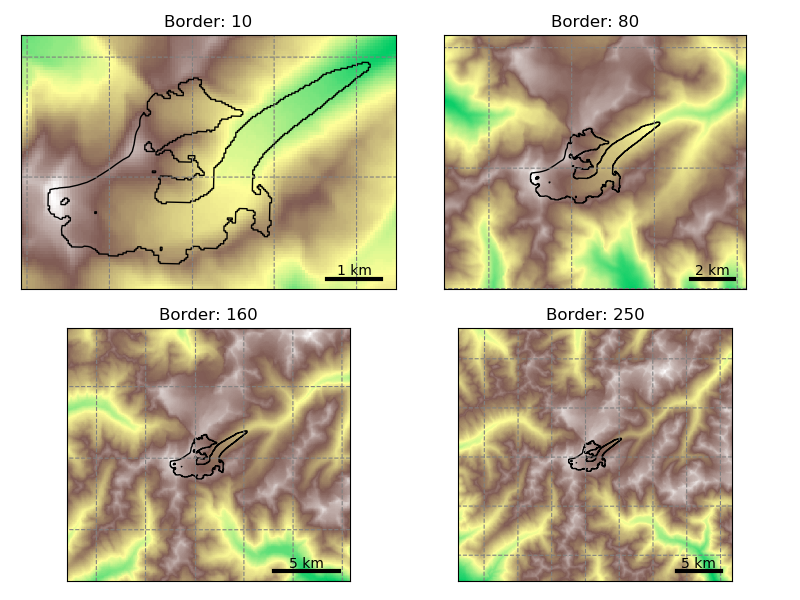
For runs into the Little Ice Age, a border value of 160 is more than enough. For simulations into the 21st century, a border value of 80 is sufficient.
Users should be aware that the amount of data to download isn’t small, especially for full directories at levels 3. Here is an indicative table for the total amount of data for all 18 RGI regions (excluding Antarctica):
| Level | B 10 | B 80 | B 160 | B 250 |
|---|---|---|---|---|
| L1 | 2.4G | 11G | 29G | 63G |
| L2 | 5.1G | 14G | 32G | 65G |
| L3 | 13G | 44G | 115G | 244G |
| L4 | 4.2G | 4.5G | 4.8G | 5.3G |
Certain regions are much smaller than others of course. As an indication, with prepro level 3 and a map border of 160, the Alps are 2G large, Greenland 11G, and Iceland 334M.
Therefore, it is recommended to always pick the smallest border value suitable for your research question, and to start your runs from level 4 if possible.
Note
The data download of the preprocessed directories will occur one single time
only: after the first download, the data will be cached in OGGM’s
dl_cache_dir folder (see above).
Raw data sources
These data are used to create the pre-processed directories explained above. If you want to run your own workflow from A to Z, or if you would like to know which data are used in OGGM, read further!
Glacier outlines and intersects
Glacier outlines are obtained from the Randolph Glacier Inventory (RGI). We recommend to download them right away by opening a python interpreter and type:
from oggm import utils
utils.get_rgi_intersects_dir()
utils.get_rgi_dir()
The RGI folders should now contain the glacier outlines in the shapefile format, a format widely used in GIS applications. These files can be read by several softwares (e.g. qgis), and OGGM can read them too.
The “RGI Intersects” shapefiles contain the locations of the ice divides (intersections between neighboring glaciers). OGGM can make use of them to determine which bed shape should be used (rectangular or parabolic). See the rgi tools documentation for more information about the intersects.
Topography data
When creating a Glacier directories a suitable topographical data source is chosen automatically, depending on the glacier’s location. Currently we use:
- the Shuttle Radar Topography Mission (SRTM) 90m Digital Elevation Database v4.1 for all locations in the [60°S; 60°N] range
- the Greenland Mapping Project (GIMP) Digital Elevation Model for mountain glaciers in Greenland (RGI region 05)
- the Radarsat Antarctic Mapping Project (RAMP) Digital Elevation Model, Version 2 for mountain glaciers in the Antarctic continent (RGI region 19 with the exception of the peripheral islands)
- the Viewfinder Panoramas DEM3 products elsewhere (most notably: North America, Russia, Iceland, Svalbard)
These data are downloaded only when needed (i.e.: during an OGGM run)
and they are stored in the dl_cache_dir
directory. The gridded topography is then reprojected and resampled to the local
glacier map. The local grid is defined on a Transverse Mercator projection centered over
the glacier, and has a spatial resolution depending on the glacier size. The
default in OGGM is to use the following rule:
where \(\Delta x\) is the grid spatial resolution (in m), \(S\) the glacier area (in km\(^{2}\)) and \(d_1\), \(d_2\) some parameters (set to 14 and 10, respectively). If the chosen spatial resolution is larger than 200 m (\(S \ge\) 185 km\(^{2}\)) we clip it to this value.
Important: when using these data sources for your OGGM runs, please refer
to the original data provider of the data! OGGM will add a dem_source.txt
file in each glacier directory specifying how to cite these data. We
reproduce this information here:
- SRTM V4
- Jarvis A., H.I. Reuter, A. Nelson, E. Guevara, 2008, Hole-filled seamless SRTM data V4, International Centre for Tropical Agriculture (CIAT), available from http://srtm.csi.cgiar.org.
- RAMP V2
- Liu, H., K. C. Jezek, B. Li, and Z. Zhao. 2015. Radarsat Antarctic Mapping Project Digital Elevation Model, Version 2. Boulder, Colorado USA. NASA National Snow and Ice Data Center Distributed Active Archive Center. doi: https://doi.org/10.5067/8JKNEW6BFRVD.
- GIMP V1.1
- Howat, I., A. Negrete, and B. Smith. 2014. The Greenland Ice Mapping Project (GIMP) land classification and surface elevation data sets, The Cryosphere. 8. 1509-1518. https://doi.org/10.5194/tc-8-1509-2014
- VIEWFINDER PANORAMAS DEMs
- There is no recommended citation for these data. Please refer to the website above in case of doubt.
Warning
A number of glaciers will still suffer from poor topographic information. Either the errors are large or obvious (in which case the model won’t run), or they are left unnoticed. The importance of reliable topographic data for global glacier modelling cannot be emphasized enough, and it is a pity that no consistent, global DEM is yet available for scientific use.
Climate data
The MB model implemented in OGGM needs monthly time series of temperature and precipitation. The current default is to download and use the CRU TS data provided by the Climatic Research Unit of the University of East Anglia.
‣ CRU (default)
If not specified otherwise, OGGM will automatically download and unpack the latest dataset from the CRU servers. We recommend to do this before your first run. In a python interpreter, type:
from oggm import utils
utils.get_cru_file(var='tmp')
utils.get_cru_file(var='pre')
Warning
While the downloaded zip files are ~370mb in size, they are ~5.6Gb large after decompression!
The raw, coarse (0.5°) dataset is then downscaled to a higher resolution grid (CRU CL v2.0 at 10’ resolution) following the anomaly mapping approach described by Tim Mitchell in his CRU faq (Q25). Note that we don’t expect this downscaling to add any new information than already available at the original resolution, but this allows us to have an elevation-dependent dataset based on a presumably better climatology. The monthly anomalies are computed following Harris et al., (2010): we use standard anomalies for temperature and scaled (fractional) anomalies for precipitation. At the locations where the monthly precipitation climatology is 0 we fall back to the standard anomalies.
When using these data, please refer to the original provider:
Harris, I., Jones, P. D., Osborn, T. J., & Lister, D. H. (2014). Updated high-resolution grids of monthly climatic observations - the CRU TS3.10 Dataset. International Journal of Climatology, 34(3), 623–642. https://doi.org/10.1002/joc.3711
‣ User-provided dataset
You can provide any other dataset to OGGM by setting the climate_file
parameter in params.cfg. See the HISTALP data file in the sample-data
folder for an example.
‣ GCM data
OGGM can also use climate model output to drive the mass-balance model. In this case we still rely on gridded observations (CRU) for the baseline climatology and apply the GCM anomalies computed from a preselected reference period. This method is sometimes called the delta method.
Currently we can process data from the
CESM Last Millenium Ensemble
project (see tasks.process_cesm_data()), but adding other models
should be relatively easy.
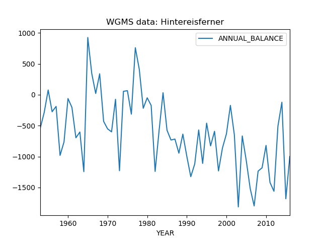
Mass-balance data
In-situ mass-balance data is used by OGGM to calibrate and validate the mass-balance model. We reliy on mass-balance observations provided by the World Glacier Monitoring Service (WGMS). The Fluctuations of Glaciers (FoG) database contains annual mass-balance values for several hundreds of glaciers worldwide. We exclude water-terminating glaciers and the time series with less than five years of data. Since 2017, the WGMS provides a lookup table linking the RGI and the WGMS databases. We updated this list for version 6 of the RGI, leaving us with 254 mass balance time series. These are not equally reparted over the globe:

Map of the RGI regions; the red dots indicate the glacier locations and the blue circles the location of the 254 reference WGMS glaciers used by the OGGM calibration. From our GMD paper.
These data are shipped automatically with OGGM. All reference glaciers have access to the timeseries through the glacier directory:
In [4]: gdir = workflow.init_glacier_regions('RGI60-11.00897', from_prepro_level=4,
   ...:                                      prepro_border=10)[0]
   ...:

In [5]: mb = gdir.get_ref_mb_data()

In [6]: mb[['ANNUAL_BALANCE']].plot(title='WGMS data: Hintereisferner')
Out[6]: <matplotlib.axes._subplots.AxesSubplot at 0x7fc44cce5cc0>