Bed inversion
To compute the initial ice thickness \(h_0\), OGGM follows a methodology largely inspired from [Farinotti_etal_2009], but fully automatised and relying on different methods for the mass-balance and the calibration.
Basics
The principle is simple. Let’s assume for now that we know the flux of ice \(q\) flowing through a section of our glacier. The flowline physics and geometrical assumptions can be used to solve for the ice thickness \(h\):
With \(n=3\) and \(S = h w\) (in the case of a rectangular section) or \(S = 2 / 3 h w\) (parabolic section), the equation reduces to solving a polynomial of degree 5 with one unique solution in \(\mathbb{R}_+\). If we neglect sliding (the default in OGGM and in [Farinotti_etal_2009]), the solution is even simpler.
Ice flux
If we consider a point on the flowline and the catchment area \(\Omega\) upstream of this point we have:
with \(\dot{m}\) the mass balance, and \(\widetilde{m} = \dot{m} - \rho \partial h / \partial t\) the “apparent mass-balance” after [Farinotti_etal_2009]. If the glacier is in steady state, the apparent mass-balance is equivalent to the the actual (and observable) mass-balance. Unfortunately, \(\partial h / \partial t\) is not known and there is no easy way to compute it. In order to continue, we have to make the assumption that our geometry is in equilibrium.
This however has a very useful consequence: indeed, for the calibration of our Mass-balance model it is required to find a date \(t^*\) at which the glacier would be in equilibrium with its average climate while conserving its modern geometry. Thus, we have \(\widetilde{m} = \dot{m}_{t^*}\), where \(\dot{m}_{t^*}\) is the 31-yr average mass-balance centered at \(t^*\) (which is known since the mass-balance model calibration).
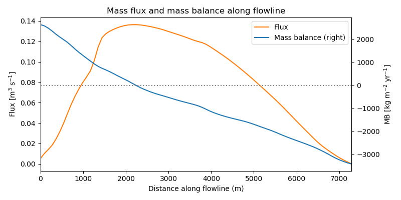
The plot below shows the mass flux along the major flowline of Hintereisferner glacier. By construction, the flux is maximal at the equilibrium line and zero at the glacier tongue.
In [1]: example_plot_massflux()
Calibration
A number of climate and glacier related parameters are fixed prior to the inversion, leaving only one free parameter for the calibration of the bed inversion procedure: the inversion factor \(f_{inv}\). It is defined such as:
With \(A_0\) the standard creep parameter (\(2.4^{-24}\)). Currently, there is no “optimum” \(f_{inv}\) parameter in the model. There is a high uncertainty in the “true” \(A\) parameter as well as in all other processes affecting the ice thickness. Therefore, we cannot make any recommendation for the “best” parameter. Global sensitivity analyses show that the default value is a good compromise (Maussion et al., 2018)
Note: for ITMIX, \(f_{inv}\) was set to a value of approximately 3 (which was too high and underestimated ice thickness in most cases with the exception of the European Alps).
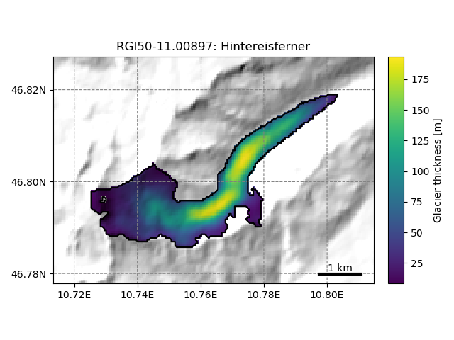
Distributed ice thickness
To obtain a 2D map of the glacier bed, the flowline thicknesses need to be interpolated to the glacier mask. The current implementation of this step in OGGM is currently very simple, but provides nice looking maps:
In [2]: tasks.catchment_area(gdir)

In [3]: graphics.plot_distributed_thickness(gdir)