OGGM Shop#
OGGM needs various data files to run. We rely exclusively on open-access data that can be downloaded automatically for the user. We like to call this service a “shop”, allowing users to define a shopping list of data that they wish to add to their Glacier directories.
This page describes the various products you will find in the shop.
Important
Don’t forget to set-up or check your system (First step: system settings for input data) before downloading new data! (you’ll need to do this only once per computer)
Pre-processed directories#
The simplest way to run OGGM is to rely on Glacier directories which have been prepared for you by the OGGM developers. Depending on your use case, you can start from various stages in the processing chain, map sizes, and model set-ups.
The directories have been generated with the standard parameters of the current stable OGGM version (and a few alternative combinations). If you want to change some of these parameters, you may have to start a run from a lower processing level and re-run the processing tasks. Whether or not this is necessary depends on the stage of the workflow you’d like your computations to diverge from the defaults (this will become more clear as we provide examples below).
To start from a pre-processed state, simply use the
workflow.init_glacier_directories() function with the
prepro_base_url, from_prepro_level and prepro_border keyword arguments
set to the values of your choice. This will fetch the desired directories:
there are more options to these, which we explain below.
Processing levels#
New in version 1.6!
Since v1.6, Level 4 and Level 5 have changed!
Currently, there are six available levels of pre-processing:
Level 0: the lowest level, with directories containing the glacier outlines only.
Level 1: directories now contain the glacier topography data as well.
Level 2: at this stage, the flowlines and their downstream lines are computed and ready to be used.
Level 3: adding the baseline climate timeseries (e.g. W5E5, CRU or ERA5) to the directories. Adding all necessary pre-processing tasks for a dynamical run, including the mass balance calibration, bed inversion, up to the
tasks.init_present_time_glacier()task included. These directories still contain all data that were necessary for the processing, i.e. large in size but also the most flexible since the processing chain can be re-run from them.Level 4: includes a historical simulation from the RGI date to the last possible date of the baseline climate file (currently January 1st 2020 at 00H for most datasets), stored with the file suffix
_historical. Moreover, some configurations (calleddynspin) may include a simulation running a spinup from 1979 to the last possible date of the baseline climate file, stored with the file suffix_spinup_historical. This spinup attempts to conduct a dynamic mu star calibration and a dynamic spinup matching the RGI area. If this fails, only a dynamic spinup is carried out. If this also fails, a fixed geometry spinup is conducted. To learn more about these different spinup types, check out Dynamic spinup.Level 5: same as level 4 but with all intermediate output files removed. The strong advantage of level 5 files is that their size is considerably reduced, at the cost that certain operations (like plotting on maps or running the bed inversion algorithm) are not possible anymore.
In practice, most users are going to use level 2, level 3 or level 5 files. To save space on our servers, level 4 data might be unavailable for some experiments (but easily recovered if needed).
Changes to the version 1.4 directories
In previous versions, level 4 files were the “reduced” directories with intermediate files removed. Level 5 was very similar, but without the dynamic spinup files. I practice, most users wont really see a change. All v1.4 directories are still working with OGGM v1.6: however, you may have to change the run parameters back to their previous values.
Here are some example use cases for glacier directories, and recommendations on which level to pick:
Running OGGM from GCM / RCM data with the default settings: start at level 5
Using OGGM’s flowlines but running your own baseline climate, mass balance or ice thickness inversion models: start at level 2 (and maybe use OGGM’s workflow again for glacier dynamic evolution?). This is the workflow used by associated model PyGEM for example.
Run sensitivity experiments for the ice thickness inversion: start at level 3 (with climate data available) and re-run the inversion steps.
Glacier map size: the prepro_border argument#
The size of the local glacier map is given in number of grid points outside the glacier boundaries. The larger the map, the largest the glacier can become. Here is an example with Hintereisferner in the Alps:
f, axs = plt.subplots(2, 2, figsize=(8, 6))
for ax, border in zip(np.array(axs).flatten(), [10, 80, 160, 240]):
    gdir = workflow.init_glacier_directories('RGI60-11.00897',
                                             from_prepro_level=1,
                                             prepro_base_url=base_url,
                                             prepro_border=border)
    graphics.plot_domain(gdir, ax=ax, title='Border: {}'.format(border),
                         add_colorbar=False,
                         lonlat_contours_kwargs={'add_tick_labels':False})
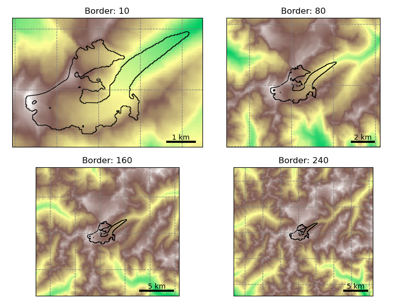
Users should choose the map border parameter depending on the expected glacier growth in their simulations. For simulations into the 21st century, a border value of 80 is sufficient. For runs into the Little Ice Age, a border value of 160 or 240 is recommended.
Users should be aware that the amount of data to download isn’t small, especially for full directories at processing level 3 and 4. Here is an indicative table for the total amount of data with ERA5 centerlines for all 19 RGI regions:
Level |
B 10 |
B 80 |
B 160 |
B 240 |
|---|---|---|---|---|
L0 |
979M |
979M |
979M |
979M |
L1 |
3.3G |
17G |
47G |
95G |
L2 |
8.3G |
49G |
142G |
285G |
L3 |
14G |
55G |
148G |
292G |
L4 |
58G |
152G |
296G |
|
L5 |
11G |
11G |
12G |
L4 and L5 data are not available for border 10 (the domain is too small for the downstream lines).
Certain regions are much smaller than others of course. As an indication, with prepro level 3 and a map border of 160, the Alps are ~2.1G large, Greenland ~21G, and Iceland ~660M.
Therefore, it is recommended to always pick the smallest border value suitable for your research question, and to start your runs from level 5 if possible.
Note
The data download of the preprocessed directories will occur one single time
only: after the first download, the data will be cached in OGGM’s
dl_cache_dir folder (see First step: system settings for input data).
Available pre-processed configurations#
OGGM has several configurations and directories to choose from, and the list is getting larger. Don’t hesitate to ask us if you are unsure about which to use, or if you’d like to have more configurations to choose from!
To choose from a specific model configuration, use the prepro_base_url
argument in your call to workflow.init_glacier_directories(),
and set it to one of the urls listed below.
As of March 10, 2023, we offer several urls. Explore https://cluster.klima.uni-bremen.de/~oggm/gdirs/oggm_v1.6 and our tutorials for examples of applications.
Version 1.4 and 1.5 directories (before v1.6)
All v1.4 directories are still working with OGGM v1.6: however, you may have to change the run parameters back to their previous values. We document them here:
A. Default
If not provided with a specific prepro_base_url argument,
workflow.init_glacier_directories() will download the glacier
directories from the default urls. Here is a summary of the default configuration:
model parameters as of the
oggm/params.cfgfile at the published model versionflowline glaciers computed from the geometrical centerlines (including tributaries)
baseline climate from CRU (not available for Antarctica) using a global precipitation factor of 2.5 (path index: pcp2.5)
baseline climate quality checked and corrected if needed with
tasks.historical_climate_qc()withN=3. If the condition of at least 3 months of melt per year at the terminus and 3 months of accumulation at the glacier top is not reached, temperatures are shifted (path index: qc3).mass balance parameters calibrated with the standard OGGM procedure (path index: no_match). No calibration against geodetic MB (see options below for regional calibration).
ice volume inversion calibrated to match the ice volume from [Farinotti_etal_2019] at the RGI region level, i.e. glacier estimates might differ. If not specified otherwise, it’s also the precalibrated parameters that will be used for the dynamical run.
frontal ablation by calving (at inversion and for the dynamical runs) is switched off
To see the code that generated these directories (for example if you want to
make your own, visit cli.prepro_levels.run_prepro_levels()
or this file on github).
The urls used by OGGM per default are in the following ftp servor:
https://cluster.klima.uni-bremen.de/~oggm/gdirs/oggm_v1.4/ :
L1-L2_files/centerlines for level 1 and level 2
L3-L5_files/CRU/centerlines/qc3/pcp2.5/no_match for level 3 to 5
If you are new to this, we recommend to explore these directories to familiarize yourself to their content. Of course, when provided with an url such as above, OGGM will know where to find the respective files automatically, but is is good to understand how they are structured. The summary folder (example) contains diagnostic files which can be useful as well.
B. Option: Geometrical centerlines or elevation band flowlines
The type of flowline to use (see Glacier flowlines) can be decided at level 2 already. Therefore, the two configurations available at level 2 from these urls:
L1-L2_files/centerlines for centerlines
L1-L2_files/elev_bands for elevation bands
The default pre-processing set-ups are also available with each of these flowline types. For example with CRU:
L3-L5_files/CRU/centerlines/qc3/pcp2.5/no_match for centerlines
L3-L5_files/CRU/elev_bands/qc3/pcp2.5/no_match for elevation bands
C. Option: Baseline climate data
For the two most important default configurations (CRU or ERA5 as baseline climate), we provide all levels for both the geometrical centerlines or the elevation band flowlines:
L3-L5_files/CRU/centerlines/qc3/pcp2.5/no_match for CRU + centerlines
L3-L5_files/CRU/elev_bands/qc3/pcp2.5/no_match for CRU + elevation bands
L3-L5_files/ERA5/centerlines/qc3/pcp1.6/no_match for ERA5 + centerlines
L3-L5_files/ERA5/elev_bands/qc3/pcp1.6/no_match for ERA5 + elevation bands
Note that the globally calibrated multiplicative precipitation factor (pcp) depends on the used baseline climate (e.g. pcp is 2.5 for CRU and 1.6 for ERA5). If you want to use another baseline climate, you have to calibrate the precipitation factor yourself. Please get in touch with us in that case!
D. Option: Mass balance calibration method
There are different mass balance calibration options available in the preprocessed directories:
no_match: This is the default calibration option. For calibration, the direct glaciological WGMS data is used and the Marzeion et al., 2012 tstar method is applied to interpolate to glaciers without measurements. With this method, the geodetic estimates are not matched.
match_geod: The default calibration with direct glaciological WGMS data is still applied on the glacier per glacier level, but on the regional level the epsilon (residual) is corrected to match the geodetic estimates from Hugonnet et al., 2021. For example:
L3-L5_files/CRU/elev_bands/qc3/pcp2.5/match_geod for CRU + elevation bands flowlines + matched on regional geodetic mass balances
L3-L5_files/ERA5/elev_bands/qc3/pcp1.6/match_geod for ERA5 + elevation bands flowlines + matched on regional geodetic mass balances
match_geod_pergla: Only the per-glacier geodetic estimates from Hugonnet et al., 2021 (mean mass balance change between 2000 and 2020) are used for calibration. The mass balance model parameter \(\mu ^{*}\) of each glacier is calibrated to match individually the geodetic estimates (using
oggm.core.climate.mustar_calibration_from_geodetic_mb()). For the preprocessed glacier directories, the allowed \(\mu ^{*}\) range is set to 20–600 (more in Monthly temperature index model calibrated on geodetic MB data). This option only works for elevation band flowlines at the moment. match_geod_pergla makes only sense without “external” climate quality check and correction (i.e. qc0) as this is already done internally. For example:L3-L5_files/CRU/elev_bands/qc0/pcp2.5/match_geod_pergla for CRU + elevation bands flowlines + matched geodetic mass balances on individual glacier level
L3-L5_files/ERA5/elev_bands/qc0/pcp1.6/match_geod_pergla for ERA5 + elevation bands flowlines + matched geodetic mass balances on individual glacier level
Warning
make sure that you use the oggm_v1.6 directory for match_geod_pergla and match_geod_pergla_massredis! In the gdirs/oggm_v1.4 folder from the OGGM server, the match_geod_pergla preprocessed directories have a minor bug in the calibration (see this GitHUB issue). This bug is removed in the latest OGGM version and the corrected preprocessed glacier directories are inside the gdirs/oggm_v1.6 folder.
E. Further set-ups
Here is a list of other available configurations at the time of writing (explore the server for more!):
L3-L5_files/CERA+ERA5/elev_bands/qc3/pcp1.6/no_match for CERA+ERA5 + elevation bands flowlines
L3-L5_files/CERA+ERA5/elev_bands/qc3/pcp1.6/match_geod for CERA+ERA5 + elevation bands flowlines + matched on regional geodetic mass balances
L3-L5_files/ERA5/elev_bands/qc3/pcp1.8/match_geod for ERA5 + elevation bands flowlines + matched on regional geodetic mass balances + precipitation factor 1.8
L3-L5_files/CRU/elev_bands/qc0/pcp2.5/match_geod for CRU + elevation bands flowlines + matched on regional geodetic mass balances + no climate quality check
L3-L5_files/CRU/elev_bands/qc0/pcp2.5/no_match for CRU + elevation bands flowlines + no climate quality check
L3-L5_files/CRU/elev_bands/qc0/pcp2.5/match_geod_pergla_massredis for CRU + elevation bands flowlines + matched on regional geodetic mass balances + mass redistribution instead of SIA (see: Mass redistribution curve model)
L3-L5_files/ERA5/elev_bands/qc0/pcp1.6/match_geod_pergla_massredis for ERA5 + elevation bands flowlines + matched on regional geodetic mass balances + mass redistribution instead of SIA
Note: the additional set-ups might not always have all map sizes available. Please
get in touch if you have interest in a specific set-up. Remember that per default, the climate quality check
and correction (oggm.tasks.historical_climate_qc()) is applied (qc3). However, if the pre-processed directory
has the path index “qc0”, it was not applied (except for match_geod_pergla where it is applied internally).
F. Error analysis and further volume and mass change comparison for different pre-processed glacier directories
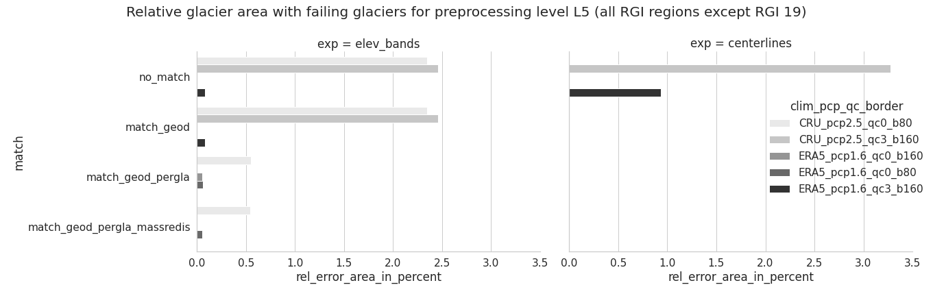
Overall, calibrating with ERA5 using a precipitation factor of 1.6 results in much less errors than CRU with pf=2.5. In addition, less errors occur for elevation bands and when using the match_geod_pergla option.#
A more detailed analysis about the type, amount and relative failing glacier area (in total and per RGI region) can be found in this error analysis jupyter notebook.
If you are also interested in how the “common” non-failing glaciers differ in terms of historical volume change, total mass change and specific mass balance between different pre-processed glacier directories, you can check out this jupyter notebook.
Climate data#
Here are the various climate datasets that OGGM handles automatically.
W5E5#
Since OGGM v1.5, users can also use the reanalysis data W5E5, which is a bias-corrected ERA5…
CRU#
CRU TS data provided by the Climatic Research Unit of the University of East Anglia. If asked to do so, OGGM will automatically download and unpack the latest dataset from the CRU servers.
Warning
While the downloaded zip files are ~370mb in size, they are ~5.6Gb large after decompression!
The raw, coarse (0.5°) dataset is then downscaled to a higher resolution grid (CRU CL v2.0 at 10’ resolution) following the anomaly mapping approach described by Tim Mitchell in his CRU faq (Q25). Note that we don’t expect this downscaling to add any new information than already available at the original resolution, but this allows us to have an elevation-dependent dataset based on a presumably better climatology. The monthly anomalies are computed following [Harris_et_al_2010] : we use standard anomalies for temperature and scaled (fractional) anomalies for precipitation.
- Harris_et_al_2010
Harris, I., Jones, P. D., Osborn, T. J., & Lister, D. H. (2014). Updated high-resolution grids of monthly climatic observations - the CRU TS3.10 Dataset. International Journal of Climatology, 34(3), 623–642. https://doi.org/10.1002/joc.3711
ERA5 and CERA-20C#
Since OGGM v1.4, users can also use reanalysis data from the ECMWF, the European Centre for Medium-Range Weather Forecasts based in Reading, UK. OGGM can use the ERA5 (1979-2019, 0.25° resolution) and CERA-20C (1900-2010, 1.25° resolution) datasets as baseline. One can also apply a combination of both, for example by applying the CERA-20C anomalies to the reference ERA5 for example (useful only in some circumstances).
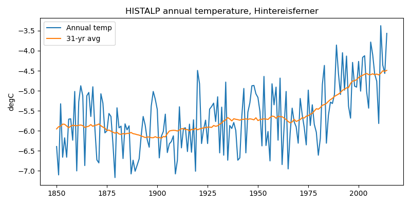
HISTALP#
If required by the user, OGGM can also automatically download and use the data from the HISTALP dataset (available only for the European Alps region, more details in [Chimani_et_al_2012]. The data is available at 5’ resolution (about 0.0833°) from 1801 to 2014. However, the data is considered spurious before 1850. Therefore, we recommend to use data from 1850 onwards.
- Chimani_et_al_2012
Chimani, B., Matulla, C., Böhm, R., Hofstätter, M.: A new high resolution absolute Temperature Grid for the Greater Alpine Region back to 1780, Int. J. Climatol., 33(9), 2129–2141, DOI 10.1002/joc.3574, 2012.
In [1]: example_plot_temp_ts() # the code for these examples is posted below
User-provided climate dataset#
You can provide any other dataset to OGGM. See the HISTALP_oetztal.nc data file in the OGGM sample-data folder for an example format.
GCM data#
OGGM can also use climate model output to drive the mass balance model. In this case we still rely on gridded observations (e.g. CRU) for the reference climatology and apply the GCM anomalies computed from a preselected reference period. This method is often called the delta method. Visit our online tutorials to see how this can be done (OGGM run with GCM tutorial).
RGI-TOPO#
The RGI-TOPO dataset provides a local topography map for each single glacier in the RGI. It was generated with OGGM, and can be used very easily from the OGGM-Shop (visit our tutorials if you are interested!).
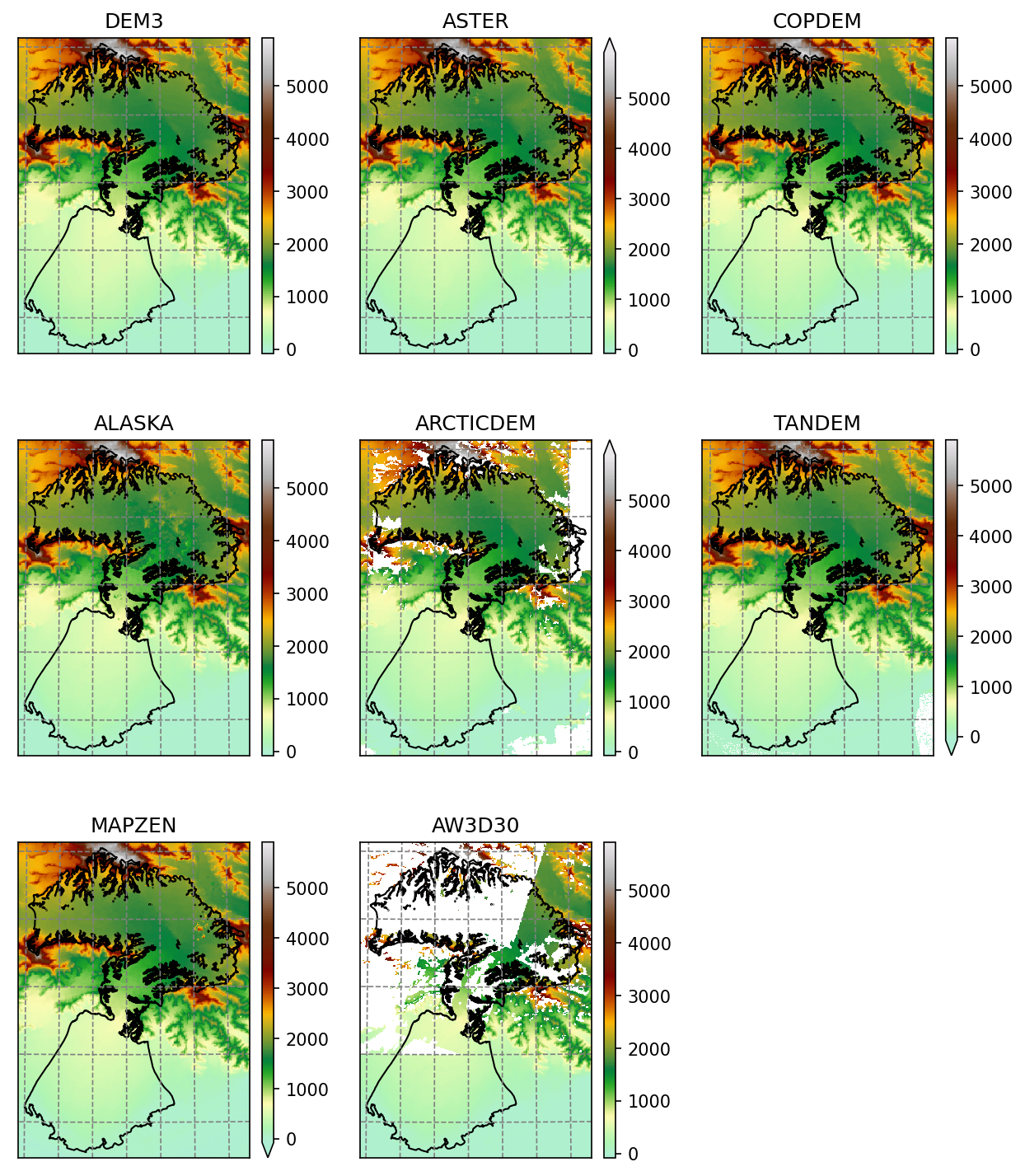
Example of the various RGI-TOPO products at Malaspina glacier#
Reference mass balance data#
Traditional in-situ MB data#
In-situ mass balance data are used by OGGM to calibrate and validate the first generation mass balance model. We rely on mass balance observations provided by the World Glacier Monitoring Service (WGMS). The Fluctuations of Glaciers (FoG) database contains annual mass balance values for several hundreds of glaciers worldwide. We exclude water-terminating glaciers and the time series with less than five years of data. Since 2017, the WGMS provides a lookup table linking the RGI and the WGMS databases. We updated this list for version 6 of the RGI, leaving us with 268 mass balance time series. These are not equally reparted over the globe:
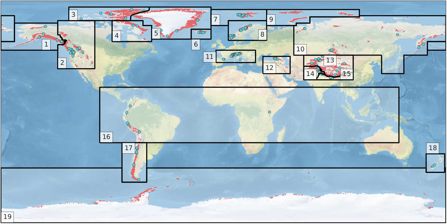
Map of the RGI regions; the red dots indicate the glacier locations and the blue circles the location of the 254 reference WGMS glaciers used by the OGGM calibration. From our GMD paper.#
These data are shipped automatically with OGGM. All reference glaciers have access to the timeseries through the glacier directory:
In [2]: base_url = 'https://cluster.klima.uni-bremen.de/~oggm/gdirs/oggm_v1.6/L3-L5_files/2023.1/elev_bands/W5E5'
In [3]: gdir = workflow.init_glacier_directories('RGI60-11.00897',
...: from_prepro_level=3,
...: prepro_base_url=base_url,
...: prepro_border=80)[0]
...:
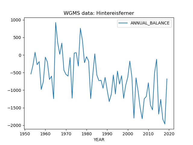
In [4]: mb = gdir.get_ref_mb_data()
In [5]: mb[['ANNUAL_BALANCE']].plot(title='WGMS data: Hintereisferner');
Geodetic MB data#
OGGM ships with a geodetic mass balance table containing MB information for all of the world’s glaciers as obtained from Hugonnet et al., 2021.
The original, raw data have been modified in three ways (code):
the glaciers in RGI region 12 (Caucasus) had to be manually linked to the product by Hugonnet because of large errors in the RGI outlines. The resulting product used by OGGM in region 12 has large uncertainties.
outliers have been filtered as following: all glaciers with an error estimate larger than 3 \(\Sigma\) at the RGI region level are filtered out
all missing data (including outliers) are attributed with the regional average.
You can access the table with:
In [6]: from oggm import utils

In [7]: mbdf = utils.get_geodetic_mb_dataframe()

In [8]: mbdf.head()
Out[8]:
                               period      area  ...  reg  is_cor
rgiid                                            ...
RGI60-01.00001  2000-01-01_2010-01-01  360000.0  ...    1   False
RGI60-01.00001  2000-01-01_2020-01-01  360000.0  ...    1   False
RGI60-01.00001  2010-01-01_2020-01-01  360000.0  ...    1   False
RGI60-01.00002  2000-01-01_2010-01-01  558000.0  ...    1   False
RGI60-01.00002  2000-01-01_2020-01-01  558000.0  ...    1   False

[5 rows x 6 columns]
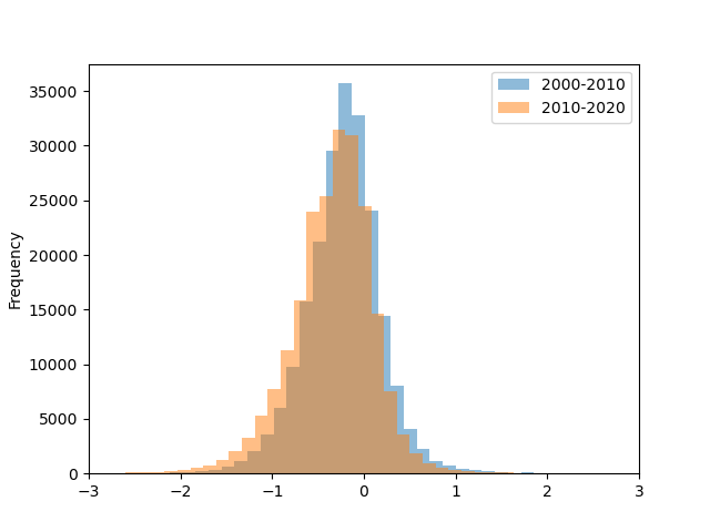
The data contains the climatic mass balance (in units meters water-equivalent per year) for three reference periods (2000-2010, 2010-2020, 2000-2020):
In [9]: mbdf['dmdtda'].loc[mbdf.period=='2000-01-01_2010-01-01'].plot.hist(bins=100, alpha=0.5, label='2000-2010');

In [10]: mbdf['dmdtda'].loc[mbdf.period=='2010-01-01_2020-01-01'].plot.hist(bins=100, alpha=0.5, label='2010-2020');

In [11]: plt.xlabel(''); plt.xlim(-3, 3); plt.legend();
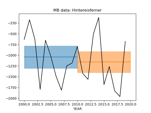
Just for fun, here is a comparison of both products at Hintereisferner:
In [12]: sel = mbdf.loc[gdir.rgi_id].set_index('period') * 1000

In [13]: _mb, _err = sel.loc['2000-01-01_2010-01-01'][['dmdtda', 'err_dmdtda']]

In [14]: plt.fill_between([2000, 2010], [_mb-_err, _mb-_err], [_mb+_err, _mb+_err], alpha=0.5, color='C0');

In [15]: plt.plot([2000, 2010], [_mb, _mb], color='C0');

In [16]: _mb, _err = sel.loc['2010-01-01_2020-01-01'][['dmdtda', 'err_dmdtda']]

In [17]: plt.fill_between([2010, 2020], [_mb-_err, _mb-_err], [_mb+_err, _mb+_err], alpha=0.5, color='C1');

In [18]: plt.plot([2010, 2020], [_mb, _mb], color='C1');

In [19]: mb[['ANNUAL_BALANCE']].loc[2000:].plot(ax=plt.gca(), title='MB data: Hintereisferner', c='k', legend=False);
ITS_LIVE#
The ITS_LIVE ice velocity products can be downloaded and reprojected to the glacier directory (visit our tutorials if you are interested!).
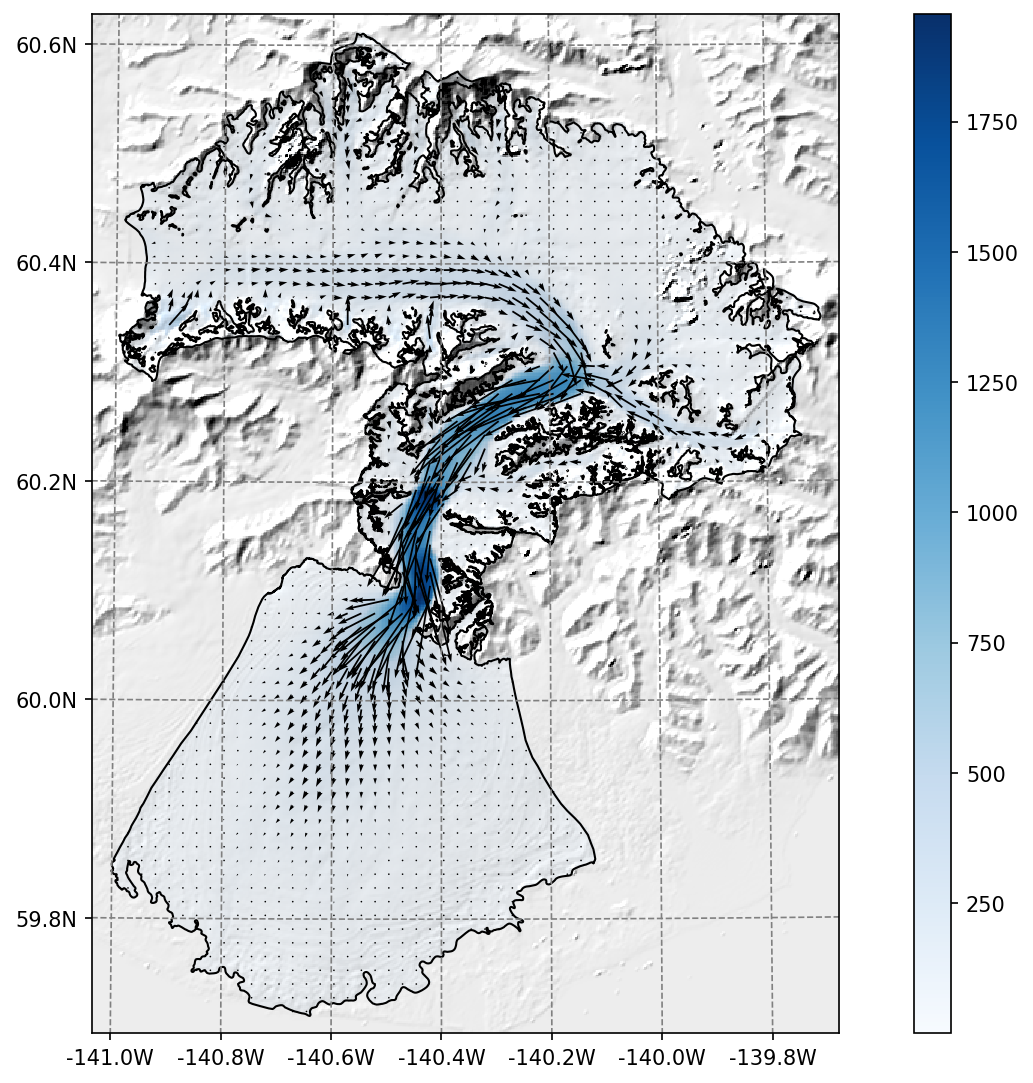
Example of the reprojected ITS_LIVE products at Malaspina glacier#
The data source used is https://its-live.jpl.nasa.gov/#data Currently the only data downloaded is the 120m composite for both (u, v) and their uncertainty. The composite is computed from the 1985 to 2018 average.
If you want more velocity products, feel free to open a new topic on the OGGM issue tracker!
Ice thickness#
The Farinotti et al., 2019 ice thickness products can be downloaded and reprojected to the glacier directory (visit our tutorials if you are interested!).
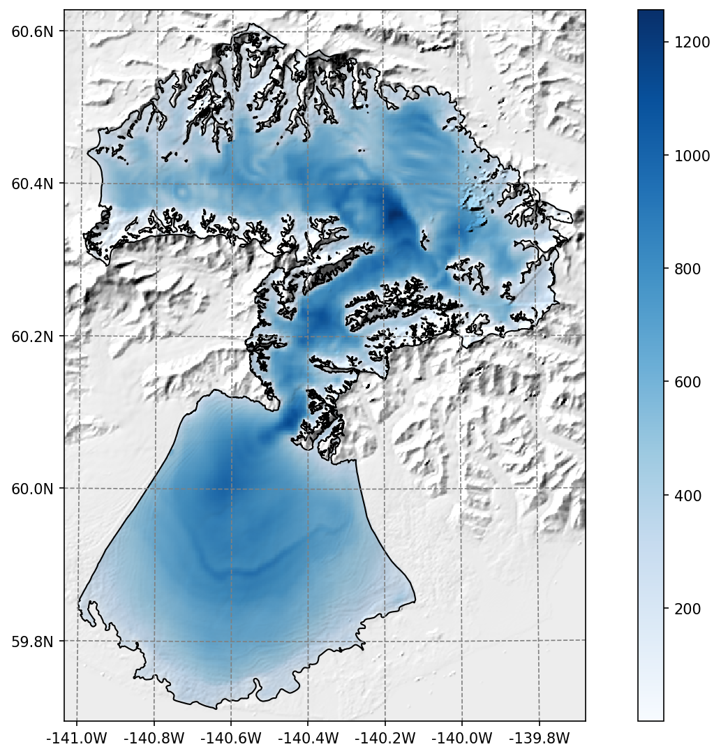
Example of the reprojected ice thickness products at Malaspina glacier#
Millan et al. (2022) ice velocity and thickness products#
Similarly, we provide data from the recent Millan et al. (2022) global study (visit our tutorials if you are interested!).
Raw data sources#
These data are used to create the pre-processed directories explained above. If you want to run your own workflow from A to Z, or if you would like to know which data are used in OGGM, read further!
Glacier outlines and intersects#
Glacier outlines are obtained from the Randolph Glacier Inventory (RGI). We recommend to download them right away by opening a python interpreter and type:
from oggm import cfg, utils
cfg.initialize()
utils.get_rgi_intersects_dir()
utils.get_rgi_dir()
The RGI folders should now contain the glacier outlines in the shapefile format, a format widely used in GIS applications. These files can be read by several software (e.g. qgis), and OGGM can read them too.
The “RGI Intersects” shapefiles contain the locations of the ice divides (intersections between neighboring glaciers). OGGM can make use of them to determine which bed shape should be used (rectangular or parabolic). See the rgi tools documentation for more information about the intersects.
The following table summarizes the RGI attributes used by OGGM. It can be useful to refer to this list if you use your own glacier outlines with OGGM.
RGI attribute |
Equivalent OGGM variable |
Comments |
|---|---|---|
RGIId |
|
|
GLIMSId |
|
not used |
CenLon |
|
|
CenLat |
|
|
O1Region |
|
not used |
O2Region |
|
not used |
Name |
|
used for graphics only |
BgnDate |
|
|
Form |
|
|
TermType |
|
|
Status |
|
|
Area |
|
|
Zmin |
|
recomputed by OGGM |
Zmax |
|
recomputed by OGGM |
Zmed |
|
recomputed by OGGM |
Slope |
|
recomputed by OGGM |
Aspect |
|
recomputed by OGGM |
Lmax |
|
recomputed by OGGM |
Connect |
not included |
|
Surging |
not included |
|
Linkages |
not included |
|
EndDate |
not included |
For Greenland and Antarctica peripheral glaciers, OGGM does not take into account the
connectivity level between the Glaciers and the Ice sheets.
We recommend to the users to think about this before they
run the task: workflow.init_glacier_directories.
Comments
- 1
The RGI id needs to be unique for each entity. It should resemble the RGI, but can have longer ids. Here are example of valid IDs:
RGI60-11.00897,RGI60-11.00897a,RGI60-11.00897_d01.- 2(1,2)
CenLonandCenLatare used to center the glacier local map and DEM.- 3
The date is the acquisition year, stored as an integer.
- 4
Glacier type:
'Glacier','Ice cap','Perennial snowfield','Seasonal snowfield','Not assigned'. Ice caps are treated differently than glaciers in OGGM: we force use a single flowline instead of multiple ones.- 5
Terminus type:
'Land-terminating','Marine-terminating','Lake-terminating','Dry calving','Regenerated','Shelf-terminating','Not assigned'. Marine and Lake terminating are classified as “tidewater” in OGGM and cannot advance - they “calve” instead, using a very simple parameterisation.- 6
Glacier status:
'Glacier or ice cap','Glacier complex','Nominal glacier','Not assigned'. Nominal glaciers fail at the “Glacier Mask” processing step in OGGM.- 7
The area of OGGM’s flowline glaciers is corrected to the one provided by the RGI, for area conservation and inter-comparison reasons. If you do not want to use the RGI area but the one computed from the shape geometry in the local OGGM map projection instead, set
cfg.PARAMS['use_rgi_area']toFalse. This is useful when using homemade inventories.
Topography data#
When creating a Glacier directories, a suitable topographical data source is chosen automatically, depending on the glacier’s location. OGGM supports a large number of datasets (almost all of the freely available ones, we hope). They are listed on the RGI-TOPO website.
The current default is to use the following datasets:
NASADEM: 60°S-60°N
COPDEM90: Global, with missing regions (islands, etc.)
GIMP, REMA: Regional datasets
TANDEM: Global, with artefacts / missing data
MAPZEN: Global, when all other things failed
These data are chosen in the provided order. If a dataset is not available, the next on the list will be tested: if the tested dataset covers 75% of the glacier area, it is selected. In practice, NASADEM and COPDEM90 are sufficient for all but about 300 of the world’s glaciers.
These data are downloaded only when needed (i.e. during an OGGM run)
and they are stored in the dl_cache_dir
directory. The gridded topography is then reprojected and resampled to the local
glacier map. The local grid is defined on a Transverse Mercator projection centered over
the glacier, and has a spatial resolution depending on the glacier size. The
default in OGGM is to use the following rule:
where \(\Delta x\) is the grid spatial resolution (in m), \(S\) the glacier area (in km\(^{2}\)) and \(d_1\), \(d_2\) some parameters (set to 14 and 10, respectively). If the chosen spatial resolution is larger than 200 m (\(S \ge\) 185 km\(^{2}\)) we clip it to this value.
Important: when using these data sources for your OGGM runs, please refer
to the original data provider of the data! OGGM adds a dem_source.txt
file in each glacier directory specifying how to cite these data. We
reproduce this information
here.
Warning
A number of glaciers will still suffer from poor topographic information. Either the errors are large or obvious (in which case the model won’t run), or they are left unnoticed. The importance of reliable topographic data for global glacier modelling cannot be emphasized enough, and it is a pity that no consistent, global DEM is yet available for scientific use. Visit rgitools for a discussion about our current efforts to find “the best” DEMs.
Note
In this blogpost we talk about which requirements a DEM must fulfill to be helpful to OGGM. And we also explain why and how we preprocess some DEMs before we make them available to the OGGM workflow.
Climate data#
‣ CRU
To download CRU data you can use the following convenience functions:
from oggm.shop import cru
cru.get_cl_file()
cru.get_cru_file(var='tmp')
cru.get_cru_file(var='pre')
Warning
While each downloaded zip file is ~200mb in size, they are ~2.9Gb large after decompression!
The raw, coarse dataset (CRU TS v4.04 at 0.5° resolution) is then downscaled to a higher resolution grid (CRU CL v2.0 at 10’ resolution) following the anomaly mapping approach described by Tim Mitchell in his CRU faq (Q25). Note that we don’t expect this downscaling to add any new information than already available at the original resolution, but this allows us to have an elevation-dependent dataset based on a presumably better climatology. The monthly anomalies are computed following Harris et al., (2010): we use standard anomalies for temperature and scaled (fractional) anomalies for precipitation. At the locations where the monthly precipitation climatology is 0 we fall back to the standard anomalies.
When using these data, please refer to the original provider:
Harris, I., Jones, P. D., Osborn, T. J., & Lister, D. H. (2014). Updated high-resolution grids of monthly climatic observations - the CRU TS3.10 Dataset. International Journal of Climatology, 34(3), 623–642. https://doi.org/10.1002/joc.3711
‣ ECMWF (ERA5, CERA, ERA5-Land)
The data from ECMWF are used “as is”, i.e. without any further downscaling.
We propose several datasets (see oggm.shop.ecmwf.process_ecmwf_data())
and, with the task oggm.tasks.historical_delta_method(), also
allow for combinations of them.
When using these data, please refer to the original provider:
For example for ERA5:
Hersbach, H., Bell, B., Berrisford, P., Biavati, G., Horányi, A., Muñoz Sabater, J., Nicolas, J., Peubey, C., Radu, R., Rozum, I., Schepers, D., Simmons, A., Soci, C., Dee, D., Thépaut, J-N. (2019): ERA5 monthly averaged data on single levels from 1979 to present. Copernicus Climate Change Service (C3S) Climate Data Store (CDS). (Accessed on < 01-12-2020 >), 10.24381/cds.f17050d7
‣ User-provided dataset
You can provide any other dataset to OGGM by setting the climate_file
parameter in params.cfg. See the HISTALP data file in the sample-data
folder for an example.
‣ GCM data
OGGM can also use climate model output to drive the mass balance model. In this case we still rely on gridded observations (CRU) for the baseline climatology and apply the GCM anomalies computed from a preselected reference period. This method is sometimes called the delta method.
Currently we can process data from the
CESM Last Millennium Ensemble
project (see tasks.process_cesm_data()), and CMIP5/CMIP6
(tasks.process_cmip_data()).