Mass-balance
The mass-balance (MB) model implemented in OGGM is an extended version of the temperature-index model presented by Marzeion et al., (2012). While the equation governing the mass-balance is that of a traditional temperature-index model, our special approach to calibration requires that we spend some time describing it.
Note
OGGM v1.4 will probably be the last model version relying on this mass-balance model only. Considerable development efforts are made to give more options to the user (see e.g. the mass-balance sandbox or PyGem, which is close to be fully compatible with OGGM).
Climate data
The MB model implemented in OGGM needs monthly time series of temperature and precipitation. The current default is to download and use the CRU TS data provided by the Climatic Research Unit of the University of East Anglia.
CRU (default)
If not specified otherwise, OGGM will automatically download and unpack the latest dataset from the CRU servers.
Warning
While the downloaded zip files are ~370mb in size, they are ~5.6Gb large after decompression!
The raw, coarse (0.5°) dataset is then downscaled to a higher resolution grid (CRU CL v2.0 at 10’ resolution) following the anomaly mapping approach described by Tim Mitchell in his CRU faq (Q25). Note that we don’t expect this downscaling to add any new information than already available at the original resolution, but this allows us to have an elevation-dependent dataset based on a presumably better climatology. The monthly anomalies are computed following [Harris_et_al_2010] : we use standard anomalies for temperature and scaled (fractional) anomalies for precipitation.
ERA5 and CERA-20C
Since OGGM v1.4, users can also use reanalysis data from the ECMWF, the European Centre for Medium-Range Weather Forecasts based in Reading, UK. OGGM can use the ERA5 (1979-2019, 0.25° resolution) and CERA-20C (1900-2010, 1.25° resolution) datasets as baseline. One can also apply a combination of both, for example by applying the CERA-20C anomalies to the reference ERA5 for example (useful only in some circumstances).
HISTALP
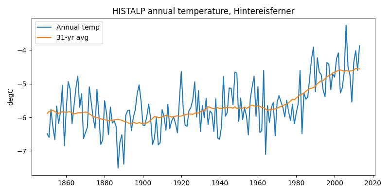
If required by the user, OGGM can also automatically download and use the data from the HISTALP dataset (available only for the European Alps region, more details in [Chimani_et_al_2012]. The data is available at 5’ resolution (about 0.0833°) from 1801 to 2014. However, the data is considered spurious before 1850. Therefore, we recommend to use data from 1850 onwards.
In [1]: example_plot_temp_ts() # the code for these examples is posted below
User-provided climate dataset
You can provide any other dataset to OGGM. See the HISTALP_oetztal.nc data file in the OGGM sample-data folder for an example format.
GCM data
OGGM can also use climate model output to drive the mass-balance model. In this case we still rely on gridded observations (e.g. CRU) for the reference climatology and apply the GCM anomalies computed from a preselected reference period. This method is often called the delta method. Visit our online tutorials to see how this can be done (OGGM run with GCM tutorial).
Elevation dependency
OGGM needs to compute the temperature and precipitation at the altitude of the glacier grid points. The default is to use a fixed lapse rate of -6.5K km \(^{-1}\) and no gradient for precipitation. However, OGGM also contains an optional algorithm which computes the local gradient by linear regression of the 9 surrounding grid points. This method requires that the near-surface temperature lapse-rates provided by the climate dataset are good (i.e. in most cases, you should probably use the simple fixed gradient instead).
Temperature-index model
The monthly mass-balance \(B_i\) at elevation \(z\) is computed as:
where \(P_i^{Solid}\) is the monthly solid precipitation, \(T_i\)
the monthly temperature and \(T_{Melt}\) is the monthly mean air
temperature above which ice melt is assumed to occur (-1°C per default).
Solid precipitation is computed out of the total precipitation. The fraction of
solid precipitation is based on the monthly mean temperature: all solid below
temp_all_solid (default: 0°C) and all liquid above temp_all_liq
(default: 2°C), linear change in between.
The parameter \(\mu ^{*}\) indicates the temperature sensitivity of the glacier, and it needs to be calibrated. \(\epsilon\) is a residual, to be determined at the calibration step.
Calibration
We will start by making two observations:
- the sensitivity parameter \(\mu ^{*}\) is depending on many parameters, most of them being glacier-specific (e.g. avalanches, topographical shading, cloudiness…).
- the sensitivity parameter \(\mu ^{*}\) will be affected by uncertainties and systematic biases in the input climate data.
As a result, \(\mu ^{*}\) can vary greatly between neighboring glaciers. The calibration procedure introduced by Marzeion et al., (2012) and implemented in OGGM makes full use of these apparent handicaps by turning them into assets.
The calibration procedure starts with glaciers for which we have direct observations of the annual specific mass-balance SMB. We use the WGMS FoG (shipped with OGGM) for this purpose.
For each of these glaciers, time-dependent “candidate” temperature sensitivities \(\mu (t)\) are estimated by requiring that the average specific mass-balance \(\overline{B_{31}}\) is equal to zero. \(\overline{B_{31}}\) is computed for a 31-year period centered around the year \(t\) and for a constant glacier geometry fixed at the RGI date (e.g. 2003 for most glaciers in the European Alps).
In [2]: example_plot_mu_ts() # the code for these examples is posted below
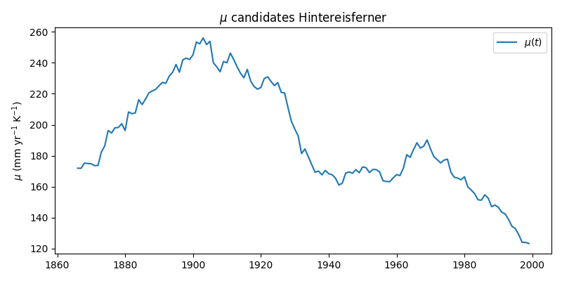
Around 1900, the climate was cold and wet. As a consequence, the temperature sensitivity required to maintain the 2003 glacier geometry is high. Inversely, the recent climate is warm and the glacier must have a small temperature sensitivity in order to preserve its 2003 geometry.
Note that these \(\mu (t)\) are just hypothetical sensitivities necessary to maintain the glacier in equilibrium in an average climate at the year \(t\). We call them “candidates”, since one (or more) of them is likely to be close to the “real” sensitivity of the glacier.
This is when the mass-balance observations come into play: each of these candidates is used to compute the mass-balance during the period were we have observations. We then compare the model output with the expected mass-balance and compute the model bias:
In [3]: example_plot_bias_ts() # the code for these examples is posted below
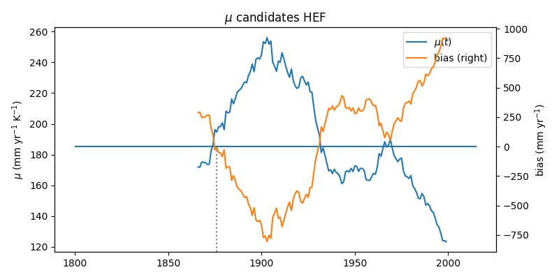
The residual bias is positive when \(\mu\) is too low, and negative when \(\mu\) is too high. Here, the residual bias crosses the zero line twice. The two dates where the zero line is crossed correspond to approximately the same \(\mu\) (but not exactly, as precipitation and temperature both have an influence on it). These two dates at which the \(\mu\) candidates are close to the “real” \(\mu\) are called \(t^*\) (the associated sensitivities \(\mu (t^*)\) are called \(\mu^*\)). For the next step, one \(t^*\) is sufficient: we pick the one which corresponds to the smallest absolute residual bias.
At the glaciers where observations are available, this detour via the \(\mu\) candidates is not necessary to find the correct \(\mu^*\). Indeed, the goal of these computations are in fact to find \(t^*\), which is the actual value interpolated to glaciers where no observations are available.
The benefit of this approach is best shown with the results of a cross-validation study realized by Marzeion et al., (2012) and confirmed by OGGM:
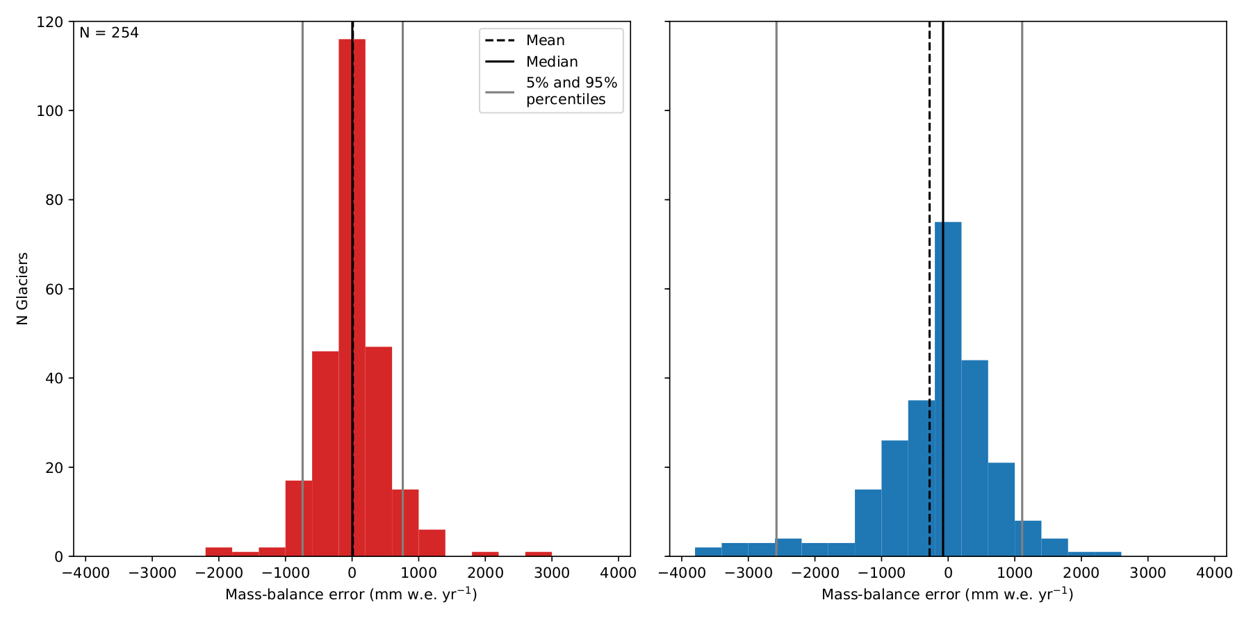
Benefit of spatially interpolating \(t^{*}\) instead of \(\mu ^{*}\) as shown by leave-one-glacier-out cross-validation (N = 255). Left: error distribution of the computed mass-balance if determined by the interpolated \(t^{*}\). Right: error distribution of the mass-balance if determined by interpolation of \(\mu ^{*}\).
This substantial improvement in model performance is due to several factors:
- the equilibrium constraint applied on \(\mu\) implies that the sensitivity cannot vary much during the last century. In fact, \(\mu\) at one glacier varies far less in one century than between neighboring glaciers, because of all the factors mentioned above. In particular, it will vary comparatively little around a given year \(t\) : errors in \(t^*\) (even large) will result in small errors in \(\mu^*\).
- the equilibrium constraint will also imply that systematic biases in temperature and precipitation (no matter how large) will automatically be compensated by all \(\mu (t)\), and therefore also by \(\mu^*\). In that sense, the calibration procedure can be seen as a empirically driven downscaling strategy: if a glacier is here, then the local climate (or the glacier temperature sensitivity) must allow a glacier to be there. For example, the effect of avalanches or a negative bias in precipitation input will have the same impact on calibration: \(\mu^*\) should be reduced to take these effects into account, even though they are not resolved by the mass-balance model.
The most important drawback of this calibration method is that it assumes that two neighboring glaciers should have a similar \(t^*\). This is not necessarily the case, as other factors than climate (such as the glacier size) will influence \(t^*\) too. Our results (and the arguments listed above) show however that this is an approximation we can cope with.
In a final note, it is important to mention that this procedure is primarily a calibration method, and as such it can be statistically scrutinized (for example with cross-validation). It can also be noted that the MB observations play a relatively minor role in the calibration: they could be entirely avoided by fixing a \(t^*\) for all glaciers in a region (or even worldwide). The resulting changes in calibrated \(\mu^*\) will be comparatively small (again, because of the local constraints on \(\mu\)). The MB observations, however, play a major role for the assessment of model uncertainty.
Regional calibration
New in version 1.4!
As of version 1.4, we now also offer to calibrate the mass-balance at the regional level (RGI regions) based on geodetic mass-balance products ([Zemp_et_al_2019] or [Hugonnet_et_al_2020]). This is done by correcting (shifting) the residual for each glacier (\(\epsilon\) in the equation above) by a constant value so that the regional estimates match the observations. This is not applied per default, as it might lead to unrealistic results at the single glacier scale (but it is very useful for global studies). An overview of the regional shifts for all regions and presently available set-ups can be assessed via this notebook.
References
| [Chimani_et_al_2012] | Chimani, B., Matulla, C., Böhm, R., Hofstätter, M.: A new high resolution absolute Temperature Grid for the Greater Alpine Region back to 1780, Int. J. Climatol., 33(9), 2129–2141, DOI 10.1002/joc.3574, 2012. |
| [Harris_et_al_2010] | Harris, I., Jones, P. D., Osborn, T. J., & Lister, D. H. (2014). Updated high-resolution grids of monthly climatic observations - the CRU TS3.10 Dataset. International Journal of Climatology, 34(3), 623–642. https://doi.org/10.1002/joc.3711 |
| [Hugonnet_et_al_2020] | Hugonnet et al., accepted. |
| [Zemp_et_al_2019] | Zemp, M., Huss, M., Thibert, E., Eckert, N., McNabb, R., Huber, J., Barandun, M., Machguth, H., Nussbaumer, S. U., Gärtner-Roer, I., Thomson, L., Paul, F., Maussion, F., Kutuzov, S. and Cogley, J. G.: Global glacier mass changes and their contributions to sea-level rise from 1961 to 2016, Nature, 568(7752), 382–386, doi:10.1038/s41586-019-1071-0, 2019. |
Implementation details
If you had the courage to read until here, it means that you have concrete questions about the implementation of the mass-balance model in OGGM. Here are some more details:
- the mass-balance in OGGM is computed from the altitudes and widths
of the flowlines grid points (see Glacier flowlines). The easiest way to let
OGGM compute the mass-balance for you is to use the
core.massbalance.PastMassBalance. - the interpolation of \(t^*\) is done with an inverse distance weighting
algorithm (see
tasks.local_t_star()) - if more than one \(t^*\) is found for some reference glaciers, than the
glaciers with only one \(t^*\) will determine the most likely \(t^*\)
for the other glaciers (see
tasks.compute_ref_t_stars()) - yes, the temperature gradients and the precipitation scaling factor will have an influence on the results, but it is small since any change will automatically be compensated by \(\mu^*\). We are currently quantifying these effects more precisely.
Code used to generate these examples:
import os
import geopandas as gpd
import matplotlib.pyplot as plt
import numpy as np
import pandas as pd
import xarray as xr

import oggm
from oggm import cfg, tasks, graphics
from oggm.core.climate import (mb_yearly_climate_on_glacier,
                               t_star_from_refmb,
                               local_t_star, mu_star_calibration)
from oggm.core.massbalance import (ConstantMassBalance)
from oggm.utils import get_demo_file, gettempdir
from oggm.shop import histalp

cfg.initialize()
cfg.set_intersects_db(get_demo_file('rgi_intersect_oetztal.shp'))
cfg.PATHS['dem_file'] = get_demo_file('hef_srtm.tif')
histalp.set_histalp_url('https://cluster.klima.uni-bremen.de/~oggm/'
                        'test_climate/histalp/')

base_dir = gettempdir('Climate_docs')
cfg.PATHS['working_dir'] = base_dir
entity = gpd.read_file(get_demo_file('Hintereisferner_RGI5.shp')).iloc[0]
gdir = oggm.GlacierDirectory(entity, base_dir=base_dir, reset=True)

tasks.define_glacier_region(gdir)
tasks.glacier_masks(gdir)
tasks.compute_centerlines(gdir)
tasks.initialize_flowlines(gdir)
tasks.compute_downstream_line(gdir)
tasks.catchment_area(gdir)
tasks.catchment_width_geom(gdir)
tasks.catchment_width_correction(gdir)
cfg.PARAMS['baseline_climate'] = 'HISTALP'
tasks.process_histalp_data(gdir)
mu_yr_clim = tasks.glacier_mu_candidates(gdir)

mbdf = gdir.get_ref_mb_data()
res = t_star_from_refmb(gdir, mbdf=mbdf.ANNUAL_BALANCE)
local_t_star(gdir, tstar=res['t_star'], bias=res['bias'], reset=True)
mu_star_calibration(gdir, reset=True)

# For flux plot
tasks.prepare_for_inversion(gdir)

# For plots
years, temp_yr, prcp_yr = mb_yearly_climate_on_glacier(gdir)

# which years to look at
selind = np.searchsorted(years, mbdf.index)
temp_yr = np.mean(temp_yr[selind])
prcp_yr = np.mean(prcp_yr[selind])

# Average oberved mass-balance
ref_mb = mbdf.ANNUAL_BALANCE.mean()
mb_per_mu = prcp_yr - mu_yr_clim * temp_yr

# Diff to reference
diff = mb_per_mu - ref_mb
pdf = pd.DataFrame()
pdf[r'$\mu (t)$'] = mu_yr_clim
pdf['bias'] = diff
res = t_star_from_refmb(gdir, mbdf=mbdf.ANNUAL_BALANCE)

# For the mass flux
cl = gdir.read_pickle('inversion_input')[-1]
mbmod = ConstantMassBalance(gdir)
mbx = (mbmod.get_annual_mb(cl['hgt']) * cfg.SEC_IN_YEAR *
       cfg.PARAMS['ice_density'])
fdf = pd.DataFrame(index=np.arange(len(mbx))*cl['dx'])
fdf['Flux'] = cl['flux']
fdf['Mass balance'] = mbx

# For the distributed thickness
tasks.mass_conservation_inversion(gdir, glen_a=2.4e-24 * 3, fs=0)
tasks.distribute_thickness_per_altitude(gdir)


# plot functions
def example_plot_temp_ts():
    d = xr.open_dataset(gdir.get_filepath('climate_historical'))
    temp = d.temp.resample(time='12MS').mean('time').to_series()
    temp.index = temp.index.year
    try:
        temp = temp.rename_axis(None)
    except AttributeError:
        del temp.index.name
    temp.plot(figsize=(8, 4), label='Annual temp')
    tsm = temp.rolling(31, center=True, min_periods=15).mean()
    tsm.plot(label='31-yr avg')
    plt.legend(loc='best')
    plt.title('HISTALP annual temperature, Hintereisferner')
    plt.ylabel(r'degC')
    plt.tight_layout()
    plt.show()


def example_plot_mu_ts():
    mu_yr_clim.plot(figsize=(8, 4), label=r'$\mu (t)$')
    plt.legend(loc='best')
    plt.title(r'$\mu$ candidates Hintereisferner')
    plt.ylabel(r'$\mu$ (mm yr$^{-1}$ K$^{-1}$)')
    plt.tight_layout()
    plt.show()


def example_plot_bias_ts():
    ax = pdf.plot(figsize=(8, 4), secondary_y='bias')
    plt.hlines(0, 1800, 2015, linestyles='-')
    ax.set_ylabel(r'$\mu$ (mm yr$^{-1}$ K$^{-1}$)')
    ax.set_title(r'$\mu$ candidates HEF')
    plt.ylabel(r'bias (mm yr$^{-1}$)')
    yl = plt.gca().get_ylim()
    plt.plot((res['t_star'], res['t_star']), (yl[0], 0),
             linestyle=':', color='grey')
    plt.ylim(yl)
    plt.tight_layout()
    plt.show()


def example_plot_massflux():
    fig, ax = plt.subplots(figsize=(8, 4))
    fdf.plot(ax=ax, secondary_y='Mass balance', style=['C1-', 'C0-'])
    plt.axhline(0., color='grey', linestyle=':')
    ax.set_ylabel('Flux [m$^3$ s$^{-1}$]')
    ax.right_ax.set_ylabel('MB [kg m$^{-2}$ yr$^{-1}$]')
    ax.set_xlabel('Distance along flowline (m)')
    plt.title('Mass flux and mass balance along flowline')
    plt.tight_layout()
    plt.show()