Bed inversion#
To compute the initial ice thickness \(h_0\), OGGM follows a methodology largely inspired from [Farinotti_et_al_2009], but fully automated and relying on different methods for the mass balance and the calibration.
Basics#
The principle is simple. Let’s assume for now that we know the flux of ice \(q\) flowing through a cross-section of our glacier. The flowline physics and geometrical assumptions can be used to solve for the ice thickness \(h\):
With \(n=3\) and \(S = h w\) (in the case of a rectangular section) or \(S = 2 / 3 h w\) (parabolic section), the equation reduces to solving a polynomial of degree 5 with one unique solution in \(\mathbb{R}_+\). If we neglect sliding (the standard in OGGM and in [Farinotti_et_al_2009]), the solution is even simpler.
Ice flux#
If we consider a point on the flowline and the catchment area \(\Omega\) upstream of this point we have:
with \(\dot{m}\) the mass balance, \(\int_{\Omega}\) the sum of all surface mass balances above the point considered, and \(\widetilde{m} = \dot{m} - \rho \partial h / \partial t\) the “apparent mass balance” after [Farinotti_et_al_2009]. If the glacier is in steady state, the apparent mass balance is equivalent to the actual (and observable) mass balance. Unfortunately, that is rarely the case, hence \(\partial h / \partial t\) is not known and there is no easy way to compute it. In order to continue, we have to make the assumption that our geometry is in equilibrium.
To do this, we create an artificial mass balance profile based on the mass balance as computed by the mass balance model. We add a residual (bias) to the 2000-2020 profile so that the specific mass balance is zero, hence following the equilibrium assumption but still being physically consistent with the original profile and mass turnover. Tests show that this method might create a slight initial shock (mostly in glacier length) during the first years of simulation, but much less than if the inversion was realized with another mass balance model or if the simulation was run from prescribed bed geometry. Therefore, each re-calibration of the mass balance model requires the inversion to be run again (more on this below).
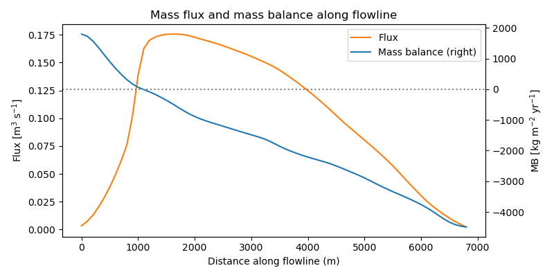
The plot below shows the mass flux along the major flowline of Hintereisferner glacier. By construction, the flux is maximal at the equilibrium line and zero at the glacier tongue.
In [1]: example_plot_massflux()
Calibration#
A number of climate and glacier related parameters are fixed prior to the inversion, leaving only one free parameter for the calibration of the bed inversion procedure: the inversion factor \(f_{inv}\). It is defined such as:
With \(A_0\) the standard creep parameter (\(2.4^{-24}\)). Currently, there is no “optimum” \(f_{inv}\) parameter in the model. There is a high uncertainty in the “true” \(A\) parameter as well as in all other processes affecting the ice thickness. Therefore, we cannot make any recommendation for the “best” parameter. Global sensitivity analyses show that the default value is a good compromise [Maussion_et_al_2019], but very likely leads to overestimated ice volume [Farinotti_et_al_2019].
New in version 1.4!
As of OGGM v1.4, the user can choose to calibrate \(A\) to match the consensus volume estimate from [Farinotti_et_al_2019] on any number of glaciers. We recommend to use a large number of glaciers (we match at the regional level) in order to allow some freedom to the model (it is not guaranteed that the consensus really is better for each glacier), but we assume that it is more accurate at large scales.
Strategies to deal with other ice thickness products#
The standard way to run OGGM is outlined above. When running OGGM from levels 3 to 5, the ice thickness has been calibrated to match the [Farinotti_et_al_2019] estimate at the regional scale, and some glaciers might experience the slight initial shock at the RGI date as explained above. For most applications, this should be fine, but as of OGGM v1.6 we also offer other tools to deal with this.
The recent Dynamic spinup capability allows two new kinds of workflow:
same as above, but preventing the initial shock thanks to spin-up (also allowing to correct for geodetic observations mismatch at the same time)
incorporating any other bed topography product into OGGM, such as [Farinotti_et_al_2019] or [Millan_et_al_2022].
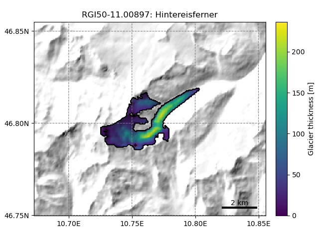
Distributed ice thickness#
To obtain a 2D map of the glacier ice thickness and bed, the flowline thicknesses need to be interpolated to the glacier mask. The current implementation of this step in OGGM is currently very simple, but provides nice looking maps:
In [2]: tasks.catchment_area(gdir)

In [3]: graphics.plot_distributed_thickness(gdir)
References#
- Farinotti_et_al_2009(1,2,3)
Farinotti, D., Huss, M., Bauder, A., Funk, M., & Truffer, M. (2009). A method to estimate the ice volume and ice-thickness distribution of alpine glaciers. Journal of Glaciology, 55 (191), 422–430.
- Farinotti_et_al_2019(1,2,3,4)
Farinotti, D., Huss, M., Fürst, J. J., Landmann, J., Machguth, H., Maussion, F. and Pandit, A.: A consensus estimate for the ice thickness distribution of all glaciers on Earth, Nat. Geosci., 12(3), 168–173, doi:10.1038/s41561-019-0300-3, 2019.
- Maussion_et_al_2019
Maussion, F., Butenko, A., Champollion, N., Dusch, M., Eis, J., Fourteau, K., Gregor, P., Jarosch, A. H., Landmann, J., Oesterle, F., Recinos, B., Rothenpieler, T., Vlug, A., Wild, C. T. and Marzeion, B.: The Open Global Glacier Model (OGGM) v1.1, Geosci. Model Dev., 12(3), 909–931, doi:10.5194/gmd-12-909-2019, 2019.
- Millan_et_al_2022
Millan, R., Mouginot, J., Rabatel, A. and Morlighem, M.: Ice velocity and thickness of the world’s glaciers, Nat. Geosci., 15(2), 124–129, doi:10.1038/s41561-021-00885-z, 2022.